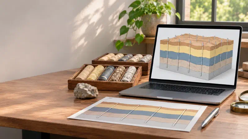
TL;DR: Want to build a 3D geological model from boreholes without writing code? A 3D geological model fills the ground with named rock layers, so you can see which layer sits where, even between drillholes. In the Geocluster workspace, three prompts to the built-in AI agent pick the boundaries between layers in 47 public South Australian holes, estimate each boundary as a surface, and fill the space between the surfaces with blocks. Then the voxel wizard loads those blocks into a 3D view you can slice. Checked against the holes, 97% of the model matches the logs.
What Is a 3D Geological Model From Boreholes?
A 3D geological model divides the ground into named units, such as a shale or a granite, with a shape between the drillholes as well as along them. You may also see this task written as 3D stratigraphic modelling, or build a 3D lithology model. Borehole and drillhole mean the same thing here. It is one task in AI for geological modelling.
A model can take three forms:
- Surfaces: one gridded surface for each boundary between units.
- Solids: closed volumes for each unit.
- A block model: small blocks, or voxels, each labelled with one unit. This guide builds one of these.
The key point is that separate surfaces do not make a valid model yet. Interpolated one at a time, two surfaces can cross, leaving a unit with negative thickness. So the surfaces must be checked, kept in order and labelled, and only then turned into volumes.
Part 1 of this series drew measured drill data in 3D cells with nothing interpolated. The previous parts matched contacts and drew a section.
The last guide showed how to interpolate geological surfaces between drillholes. In this 3D geological modelling tutorial, we combine all the surfaces into one model.
Drillhole Data Used in This Guide
We continue in the Geocluster project from the previous guide, with the same 49 holes from the SARIG Data Package, the South Australian government’s public export of drilling records. The model uses 47 of them: CAR001 has no collar elevation, and CAR041 is drilled at −60°. That project already holds the C4 picks and the kriging settings.
Download and Filter the SARIG Files
To start from scratch, download the three full exports:
- sarig_dh_details_exp.csv (140 MB): position, elevation and depth of each hole
- sarig_dh_litho_exp.csv (402 MB): the rock intervals
- sarig_dh_strat_exp.csv (58 MB): the named unit intervals
In the details export, keep the holes with ZONE_GDA2020 53, EASTING_GDA2020 from 735,000 to 741,000, NORTHING_GDA2020 from 6,543,000 to 6,546,000 and STRAT_LOG equal to Y. Then keep the rows of those 49 DRILLHOLE_NO values in the other two exports, and save the files as sarig_area_details.csv, sarig_area_litho.csv and sarig_area_strat.csv. These exports are large, so use a script or a tool built for large CSV files.
Source: The Department for Energy and Mining, the Government of South Australia, The SARIG Data Package, Sourced on 9 November 2026, https://dem-sdp.s3-ap-southeast-2.amazonaws.com/index.html.
Licensed under CC BY 4.0. We filtered the exports to 49 holes and derived the figures and the model in this guide from them. The Government of South Australia does not endorse this guide.
The model has five units, separated by four contacts, from top to bottom:
| Unit | Top contact |
|---|---|
| Simmens Quartzite Member | Ground |
| Corraberra Sandstone Member | C1 |
| Tregolana Shale Member | C2 |
| Whyalla Sandstone | C3 |
| Donington Suite (granite) | C4 |
How Do I Build a 3D Geological Model From Boreholes in Geocluster?
To build a 3D geological model from boreholes, send three prompts one at a time in the same conversation, then run the voxel wizard and view the result. Wait until each prompt finishes, and keep the browser tab open while it runs.
Step 1: Pick Every Contact in Every Hole
C4 already exists from the previous guide. This prompt takes C1, C2 and C3 from the stratigraphic log and flags every pick that the rock log does not support:
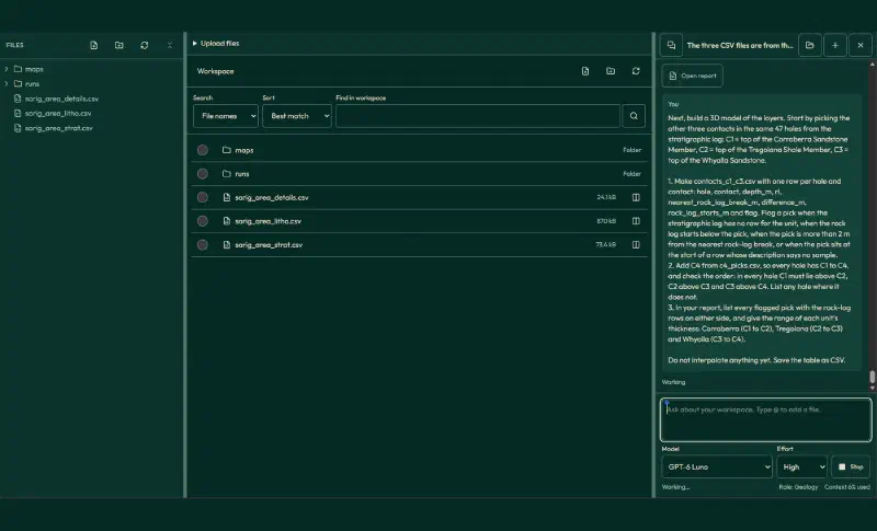
Next, build a 3D model of the layers. Start by picking the other three contacts in the same 47 holes from the stratigraphic log: C1 = top of the Corraberra Sandstone Member, C2 = top of the Tregolana Shale Member, C3 = top of the Whyalla Sandstone.

1. Make contacts_c1_c3.csv with one row per hole and contact: hole, contact, depth_m, rl, nearest_rock_log_break_m, difference_m, rock_log_starts_m and flag. Flag a pick when the stratigraphic log has no row for the unit, when the rock log starts below the pick, when the pick is more than 2 m from the nearest rock-log break, or when the pick sits at the start of a row whose description says no sample.
2. Add C4 from c4_picks.csv, so every hole has C1 to C4, and check the order: in every hole C1 must lie above C2, C2 above C3 and C3 above C4. List any hole where it does not.
3. In your report, list every flagged pick with the rock-log rows on either side, and give the range of each unit's thickness: Corraberra (C1 to C2), Tregolana (C2 to C3) and Whyalla (C3 to C4).

Do not interpolate anything yet. Save the table as CSV.
The table has 188 rows, four contacts for each of 47 holes. We checked every depth and elevation against the source files, and they all match. The order is right in every hole, and the agent flagged these picks:
| Contact | Flagged | Main reasons |
|---|---|---|
| C1 | 7 | The rock log starts deeper, so only the stratigraphic log covers the pick |
| C2 | 9 | The same 7 holes, plus CAR024 and CAR032, where the rock log disagrees |
| C3 | 10 | Two picks at 390 m that start an unsampled interval, five picks 3.5 to 39.6 m from the rock log, two where the rock log starts deeper, and CAR028 with no Whyalla row |
Step 2: Review the Picks and Interpolate Every Surface
We decided each flagged pick, keeping the choices from the earlier guides where the same hole appears. This prompt records those decisions, then interpolates the ground surface and C1 to C3 with the same kriging as C4:
I reviewed the flagged picks as the geologist. Use these decisions and accept every other pick:
- C1 and C2 in CAR038, CAR046, CAR049, CAR050, CAR051, CAR053 and CAR057: accept the stratigraphic log picks, because their rock logs start deeper.
- C2 in CAR024: keep 115 m, because its rock log has one undescribed shale row from 95.6 to 424.3 m. C2 in CAR032: use 121 m, the base of the logged sandstone.
- C3: use the base of the long shale in CAR040 (396.5 m), CAR042 (394.4 m) and CAR043 (398.2 m). Use 404.5 m in CAR028, where the rock log shows the shale ending although the stratigraphic log has no Whyalla row. Accept CAR051 (399 m) and CAR053 (393 m) from the stratigraphic log.
- Leave C3 unplaced in CAR021 and CAR024 (more than 20 m from the rock log), CAR025 and CAR026 (the pick starts an unsampled interval) and CAR049 (its rock log starts at the pick, inside siltstone).

1. Make final_contacts.csv with hole, contact, depth_m, rl and decision for C1 to C4.
2. Interpolate C1, C2 and C3 with ordinary kriging on the same 10 m grid as C4, and interpolate the ground surface from collar_rl the same way. Fit each variogram as for C4: an experimental semivariogram with 100 m lags up to 1,000 m and a spherical model fitted to those lag bins by least squares, with the nugget limited to at most 20% of the sill. Report each fit, and check that every grid varies: report its standard deviation within the mask next to the standard deviation of its picks.
3. Check the order cell by cell within 250 m of a hole: ground above C1, C1 above C2, C2 above C3 and C3 above C4. Report how many cells break each rule and by how much. Then reconcile: wherever a surface lies above the one over it, move it down to that surface, so no unit has negative thickness. Report how many cells changed.
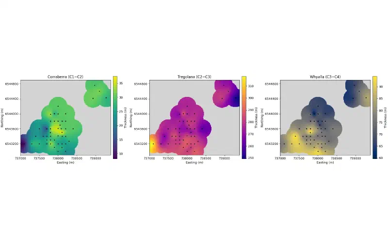
4. Draw unit_thickness.png at exactly 1800 x 1092 pixels: three maps side by side for Corraberra (C1 to C2), Tregolana (C2 to C3) and Whyalla (C3 to C4) after reconciling, with the 250 m grey mask, the holes as black dots, equal axis scales and plain tick labels, each with its own colour bar. No figure title.
5. Save the reconciled surfaces as model_surfaces.csv with easting, northing, ground_rl, c1_rl, c2_rl, c3_rl and c4_rl.

Report only values computed in code in this run. Save the tables as CSV and the figure as PNG.
The variation check matters. In our first run, every variogram fit put the whole sill into the nugget, so kriging returned the average everywhere and all four surfaces came out flat. Flat surfaces never cross, so the order check passed anyway. Comparing each grid’s spread with its picks exposed the problem at once:
| Surface | Picks, standard deviation (m) | Grid within 250 m, standard deviation (m) |
|---|---|---|
| Ground | 8.50 | 11.32 |
| C1 | 16.66 | 22.37 |
| C2 | 18.02 | 24.43 |
| C3 | 16.57 | 19.89 |
With the corrected fits, every model has a nugget of 0, and every range sits at the 10,000 m fitting limit, just like C4. We recomputed all four surfaces ourselves with those fits, and they match the agent’s grids.
No cell breaks the order, so reconciling changed nothing. The thinnest unit, Corraberra, still measures 8.1 m in the grid near CAR022, so the surfaces have room to stay apart. With thinner units or sparser holes, the same check often finds crossings, which is why it stays in the prompt.
| Unit | Thinnest in the grid (m) | Thickest in the grid (m) |
|---|---|---|
| Corraberra | 8.1 | 37.6 |
| Tregolana | 249.2 | 318.1 |
| Whyalla | 59.6 | 94.4 |
Step 3: Build the Block Model and Check It Against the Holes
Next, the agent fills the ground with 40 m by 40 m by 10 m blocks and labels each block by the surfaces above and below it. It then checks the result against every hole and writes a compact file for the Geocluster voxel wizard:
Next, turn the reconciled surfaces in model_surfaces.csv into a 3D block model of named units.

1. Make model_blocks.csv on a grid of 40 m by 40 m by 10 m blocks covering easting 737,000 to 739,400, northing 6,542,900 to 6,544,900 and RL -500 m to +130 m. For each block, take the surfaces at the block centre (the nearest 10 m surface cell) and assign: above the ground surface = empty; ground to C1 = Simmens Quartzite Member; C1 to C2 = Corraberra Sandstone Member; C2 to C3 = Tregolana Shale Member; C3 to C4 = Whyalla Sandstone; below C4 = Donington Suite. Leave blocks empty where the horizontal distance from the block centre to the nearest hole collar is more than 250 m, the same mask as the surfaces. Columns: x_index, y_index and z_index (all starting at 0, with z_index 0 at the bottom), easting, northing and rl of the block centre, and unit.
2. Check the model against the holes: for each hole, step down its final contacts every 10 m from the collar to RL -500 m, compare the unit from the contacts with the unit of the block that contains that point, and report the share that match per unit and overall, with the five holes that match least. Skip depths where a contact needed to name the unit is unplaced.
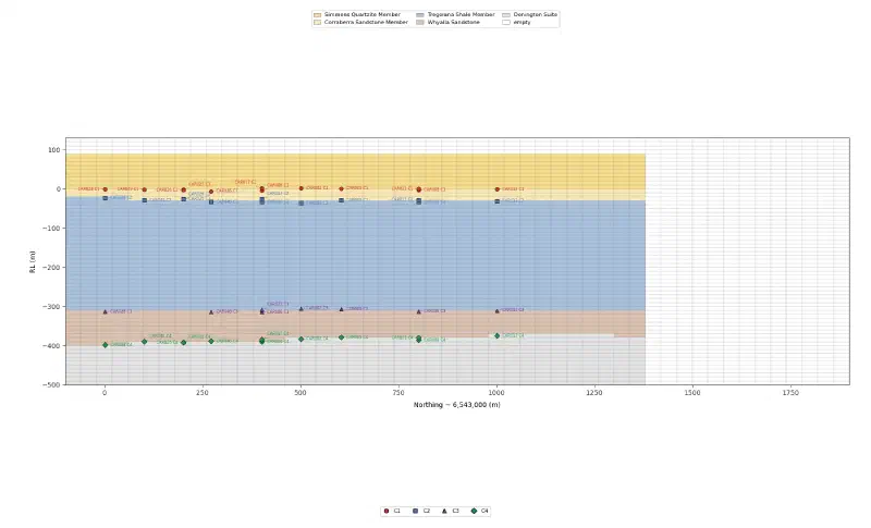
3. Draw model_section.png at exactly 1800 x 1092 pixels: a vertical slice of the block model along easting 738,200 (the column of blocks whose centres are nearest that line), with distance north of 6,543,000 on the horizontal axis and RL on the vertical axis at true scale, coloured by unit, and the final C1 to C4 picks of the holes within 100 m of the line as labelled points. Colours: Simmens #F6DC8B, Corraberra #F9E7B5, Tregolana #A9C1DC, Whyalla #D9C2B0, Donington #E3E3E3. No figure title.
4. Report the number of blocks per unit and the number of empty blocks.
5. Make model_blocks_voxel.csv for the Geocluster voxel import: only the columns x_index, y_index, z_index and unit, only the blocks that are not empty, and the unit labels renamed so they sort from top to bottom: U1 Simmens Quartzite, U2 Corraberra Sandstone, U3 Tregolana Shale, U4 Whyalla Sandstone, U5 Donington Suite.

Report only values computed in code in this run. Save the tables as CSV and the figure as PNG.
The grid has 60 × 50 × 63 = 189,000 blocks, and 80,892 of them hold a unit:
| Unit | Blocks | Match with the holes |
|---|---|---|
| Simmens | 13,525 | 94.0% |
| Corraberra | 3,771 | 88.7% |
| Tregolana | 37,757 | 98.9% |
| Whyalla | 10,502 | 96.0% |
| Donington | 15,337 | 98.7% |
Overall, 97.1% of 2,681 points down the holes match their block. Most misses sit within one block of a contact, and the thin Corraberra loses the most, because a 10 m block cannot follow an 8 m unit.
The block counts are a second safety check. In our first run, the agent measured the 250 m mask in 3D from the collar points, so blocks deeper than about 250 m below the collars came out empty, and Whyalla and Donington had zero blocks. A unit with no blocks is a clear sign of a bug, so read the counts before you open the model.
Step 4: Open the Model in 3D
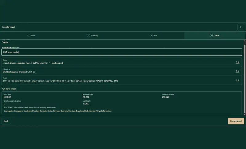
Open model_blocks_voxel.csv, tick First record contains headers and click Create voxel. The compact file matters. The full table with its empty blocks has 189,000 rows. In our run, the file view captured only part of it, and the wizard could not read the table.
In the wizard, use these settings:
| Setting | Value |
|---|---|
| Table meaning | Existing grid |
| Header rows | 1, whole table |
| Index X, Y, Z | x_index, y_index, z_index |
| Value | unit, field name Unit, Categories |
| Cells along X, Y, Z | 60, 50, 63 |
| First index | 0 |
| Empty cells | Allow empty cells |
| Coordinates | Physical coordinates, metres, Projected CRS |
| CRS | EPSG:7853 |
| Elevation reference | Collar RL, SARIG |
| Lower corner X, Y, Z | 737000, 6542900, -500 |
| Cell size X, Y, Z | 40, 40, 10 |
| Voxel name | CAR layer model |
Two settings need care:
- Cells along X, Y and Z: type them in. The file holds no empty blocks, so a size suggested from the largest index can miss empty outer layers.
- Lower corner: it is the outer corner of the first cell, not its centre.
The full-data check then reports 189,000 grid cells, 80,892 supplied and valid, and 108,108 absent, which become empty cells.
Step 5: View and Slice the Model
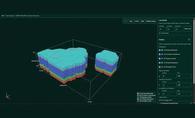
Click Create voxel and open the result in 3D. Geocluster picks each category colour from the label text. With the full SARIG names, three units came out in similar greens. The U1 to U5 labels give five distinct colours and a legend in order from top to bottom.
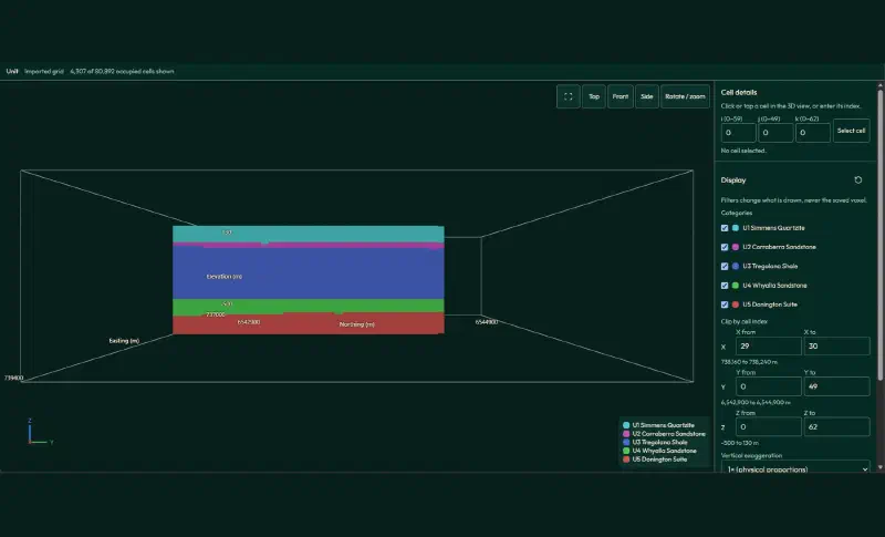
To slice the model, set X from 29 to 30 (easting 738,160 to 738,240 m) and click Side. This north-south slice, 4,307 blocks, follows the section line from the earlier guide.
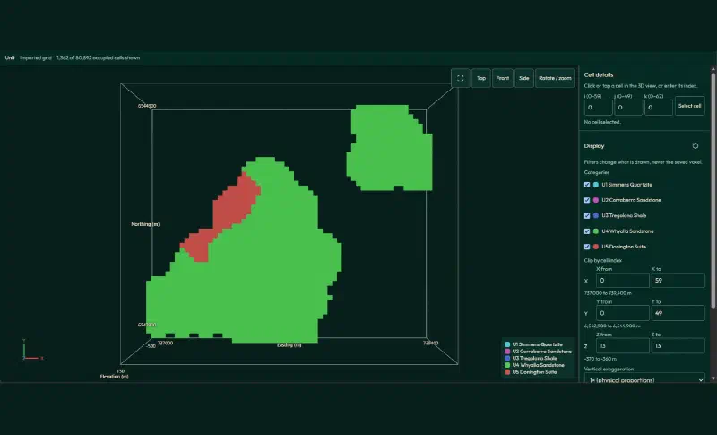
For a level map, set Z from 13 to 13 (RL −370 m to −360 m) and click Top. At this level, 1,254 blocks are Whyalla Sandstone and 108 are already granite of the Donington Suite, in a band in the north-west, where the top of the granite sits highest.
What the 3D Model Shows
Read together, the steps give a short geological picture:
- A layered cover. Four sedimentary units lie close to flat over granite, as the section in the earlier guide suggested.
- Units that change thickness. Toward CAR022 in the west, Corraberra thins to 8.1 m and Tregolana thickens to 318.1 m. Whyalla ranges from 59.6 m near CAR033 to 94.4 m near CAR056.
- A granite high. The top of the granite rises in the north-west, so it reaches RL −370 m there while Whyalla still fills that level elsewhere.
- A model that fits the holes. 97.1% of the points down the holes match their block.
Limits of a 3D Geological Model From Boreholes
When you build a 3D geological model from boreholes this way, the result carries these limits:
- Surfaces from one method. Every surface comes from ordinary kriging with a variogram whose range sits at the fitting limit. A different method would move the contacts, most of all away from holes.
- Masked, not modelled. Blocks more than 250 m from a hole stay empty. The model says nothing there.
- Block size. A 10 m block cannot follow a unit as thin as 8 m, so thin units lose detail.
- No faults, no breccia. The model assumes continuous layers. It does not include faults, and it treats the Donington Suite as one unit, without the breccia zone from the earlier section.
- Picks first. Five C3 picks stay unplaced, and several upper contacts rest on the stratigraphic log alone.
- Labels set the colours. In Geocluster, the label text decides each category colour, so we renamed the units for the 3D view.
- Yearly updates. The SARIG package changes each year, so a later download may not match the numbers here, which come from the package sourced on 9 November 2026.
- Check the written summary. Treat the saved tables and figures as the result, and verify historical drilling data against its source. We recomputed the picks, the surfaces, the block counts and the match with the holes from the source files.
FAQs
What is a 3D geological model used for?
A 3D geological model shows where each rock unit sits, including between drillholes. Geologists use it to plan new holes, to draw sections, to estimate the volume of a unit, and as the frame that keeps grade estimates inside the right rock. It is only as reliable as the contacts and the method behind it.
What is the difference between a block model and a surface model?
A surface model stores each boundary between units as a gridded surface. A block model divides the ground into small blocks and gives each one a single unit. Surfaces keep sharp contacts, while blocks are easy to slice, count and combine with other data, but they blur anything thinner than a block.
How do you stop interpolated surfaces from crossing?
Check the order of the surfaces cell by cell. Wherever a lower surface rises above the one over it, move it down to meet that surface, so the unit between them has zero thickness, not a negative one. Another way is to interpolate unit thicknesses, set negative values to zero and stack them down from the top surface.
How big should the blocks in a 3D geological model be?
Small enough to show the thinnest unit you care about, and large enough for the data and the software. Here, 40 m by 40 m by 10 m blocks matched 97% of the hole data, but the 8 m to 38 m Corraberra unit matched only 89%. Thinner blocks follow thin units better, at the cost of many more blocks.
How do you check a 3D geological model against drillholes?
Step down each hole at a fixed interval, read the unit the logs give at each point, and compare it with the model block at the same place. Report the match per unit and per hole. Also read the block counts, because a unit with no blocks usually means a bug, not geology.
Can a 3D geological model include faults?
Yes, but not with one continuous surface per contact. Faults are modelled as surfaces of their own that split the area into blocks, and each block gets its own contact surfaces. Implicit modelling tools can build these blocks for you. Before adding faults, check in sections whether the contacts really step across them.
Build a 3D Geological Model in Geocluster
Open the Geocluster web workspace to build a 3D geological model from boreholes in your browser, without writing code or setting up servers. Continue from your contact picks (or your own logs), send the three prompts above, and load the block model with the voxel wizard. You get checked surfaces, a block model that matches the holes, and a 3D view you can slice.