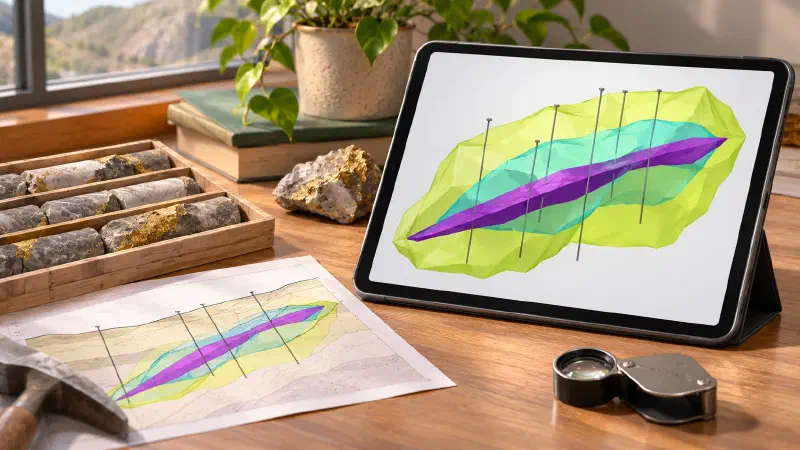
TL;DR: Want to create grade shells from drillholes without writing code? A grade shell is a 3D outline around the rock that is likely richer than a chosen grade, such as 1 gram of gold per tonne. A mineralized zone is the body of rich rock you trace from hole to hole. In the Geocluster workspace, four prompts to the built-in AI agent find the rich stretches in 80 Western Australian drillholes. They then draw shells at two grades and link the holes into one zone about 5 m thick. Finally, the voxel wizard and the map show the result in 3D and from above.
What Does It Mean to Create Grade Shells?
To create grade shells is to outline, in 3D, the rock that is probably above a cut-off grade. A grade shell is not a geological unit; it is a boundary drawn from assays. You may also see the task written as model mineralization from drillholes, mineralized zone modeling or 3D orebody modeling.
There are three common ways to draw the outline:
- Cut the grade model: keep every estimated block at or above the cut-off.
- Indicator shell: turn each sample into 1 (above the cut-off) or 0, interpolate those values, and keep the blocks where the chance of being above is 50% or more.
- Linked intercepts: mark the rich stretch in each hole, then join the tops and the bottoms from hole to hole into one zone.
Implicit geological modelling tools draw the same outlines as smooth surfaces. Here we build all three with an AI agent and compare them on the gold grade model from the previous guide.
Drillhole Data Used in This Guide
We continue in the Geocluster project of the previous guide, with the 80 Goanna holes from open-file WAMEX report A114051, from Central Laverton in Western Australia. To start from scratch, download drilling.zip from the report’s Document List tab and follow the previous guide.
Four files from the grade interpolation guide matter here:
goanna_domain_composites.csv: the 1 m gold composites, with their distance to the alteration planegoanna_domain_plane.csv: the plane through the logged alteration, dipping about 21° to the east-north-eastgoanna_block_model.csv: the 10 m × 10 m × 5 m blocks with the inverse distance gradeau_idwCL_WADL4_GEOL2017A.txt: the raw geology log from the archive
The report describes the target. At Goanna, gold sits mostly in coarser sedimentary rock, in a zone about 5 m thick and up to 15 m thick. The zone follows a reverse fault that dips moderately east.
How Do I Create Grade Shells From Drillholes in Geocluster?
To create grade shells from drillholes, open a new conversation in the same project with the + button in the agent panel. Then send four prompts one at a time. Wait until each prompt finishes, and keep the browser tab open while it runs. After that, load the result with the voxel wizard and the map.
Step 1: Find the Mineralized Intercepts in Each Hole
An intercept is a stretch of hole above a cut-off. We use 0.5 g/t, a minimum length of 2 m, and at most 2 m of poorer rock inside. The rich stretch with the most gram-metres (grade times length) is each hole’s main intercept.
This continues the gold grade model of the Goanna holes from WAMEX report A114051. Use these files from the previous guide in this project, and do not change them: goanna_domain_composites.csv (1 m composites with distance_m to the alteration plane and in_domain), goanna_domain_plane.csv (the plane), goanna_block_model.csv (10 m × 10 m × 5 m blocks with au_idw) and CL_WADL4_GEOL2017A.txt (the raw geology log: the row starting with H1000 holds the column names, rows starting with D hold the data, tab-separated Latin-1 text).

1. Find the mineralised intercepts in each hole from the composites, using the uncapped au_ppm. Start at a composite at or above 0.5 g/t and extend down the hole while the next composite is contiguous (its from_m equals the previous to_m). Allow at most 2 consecutive composites below 0.5 g/t inside an intercept, and end it at the last composite at or above 0.5 g/t. Keep intercepts at least 2 m long (to_m minus from_m). For each intercept give hole_id, from_m, to_m, length_m, the grade weighted by sampled_length_m, gram-metres (grade × length_m), the highest composite, the mean distance_m of its composites, and the share of its composites inside the domain.
2. Mark the main intercept of each hole, the one with the most gram-metres. Report the number of intercepts, the number of holes with at least one, the median and mean length of the main intercepts, and the share of all composite gold (au_ppm × sampled_length_m) that lies inside intercepts.
3. For every composite, look up Lithology1, Alt1_Mineral and Alt2_Mineral at its midpoint depth in CL_WADL4_GEOL2017A.txt, using only rows with a Lithology1 code. Report, for composites inside intercepts and for all composites, the share of each Lithology1 code and the share with ASMS in Alt1_Mineral or Alt2_Mineral.
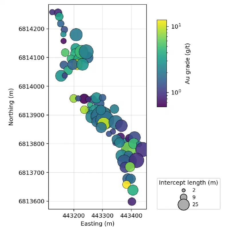
4. Draw main_intercepts.png at exactly 1800 x 1092 pixels: a plan view on equal-scale axes with full coordinates (no offset or scientific notation), limited to the data plus a small margin, with one circle per main intercept at the mean position of its composites, coloured by grade on a logarithmic scale in g/t and sized by length. Keep both axis labels visible and place the colour bar and the size legend right beside the map. No figure title.

Report only values computed in code in this run. Save the intercepts as CSV and the figure as PNG under new file names.
The agent found 97 intercepts in 73 of the 80 holes. Main intercepts are 6 m long at the median and 6.6 m on average, close to the 5 m in the report. The intercepts hold about 16% of the composites but 86.7% of the gold. The best is GDDH0101: 10 m at 9.67 g/t from 184.2 m, or 96.7 gram-metres.
The rock inside the intercepts tells the same story as the report:
| Rock code (name) | Inside intercepts | All composites |
|---|---|---|
| SAN (Arenite) | 41.7% | 30.6% |
| SAG (Argillite) | 44.9% | 54.8% |
| SMP (polymict conglomerate) | 7.3% | 4.9% |
| SIF (Banded Iron Formation) | 1.3% | 2.7% |
Logged ASMS alteration | 45.6% | 12.1% |
Coarse arenite and conglomerate are richer in intercepts, and the silica and sericite alteration is almost four times as common. Banded iron formation is rarer inside the intercepts. So the gold seems to sit near the BIF rather than in it. That fits the report, whose best grades occur where the fault meets BIF in the hanging wall.
Step 2: Build Grade Shells by Indicator Interpolation
An indicator shell asks a yes or no question at each block: is it likely above the cut-off? We use the same search as the grade model, so the shells follow the zone along strike.
Next, build grade shells by indicator interpolation, in the same blocks as the grade model.

1. For the domain composites (in_domain true), set an indicator to 1 where au_ppm is at or above 0.3 g/t and 0 otherwise. Do the same for 1 g/t.
2. Interpolate each indicator to the centre of every block in goanna_block_model.csv by inverse distance squared, with the search of the grade model. Rotate coordinates into the frame of the plane in goanna_domain_plane.csv: along strike (dip direction minus 90°), down dip within the plane, and across the plane. Divide those three distances by 70, 50 and 10 m, and use the composites within 1.5 in those units: at most 24, at most 6 from one hole, and at least 4 from at least 2 holes (leave the block empty otherwise). The result is the probability that the block is at or above the cut-off.
3. A shell is the set of blocks with a probability of 0.5 or more. For each cut-off, report the number of shell blocks and their volume at 500 m³ per block, and for comparison the number of blocks with au_idw at or above the cut-off. Place each domain composite in the block that contains its midpoint, and report the share of the domain composites at or above the cut-off that fall in shell blocks, the share of the domain gold (au_ppm × sampled_length_m) in shell blocks, and the mean grade of the composites in shell blocks.
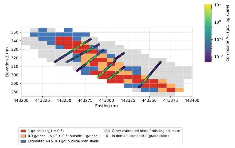
4. Draw shells_section.png at exactly 1800 x 1092 pixels: an east-west section of the blocks with y_index 29 to 31 (northing 6,813,870 to 6,813,900), with east on the horizontal axis and z on the vertical axis at equal scale, and full coordinates. For each x_index and z_index, colour the cell by the highest class among those three rows: 1 g/t shell, 0.3 g/t shell, au_idw at or above 0.3 g/t but outside both shells, other estimated block. Add the domain composites within those northings as points coloured by grade on a logarithmic scale in g/t. No figure title.

Report only values computed in code in this run. Save the block probabilities as CSV with x_index, y_index, z_index, p_03 and p_1, and every figure as PNG under a new file name.
| Cut-off | Shell blocks | Volume (m³) | Blocks with au_idw at or above | Composites above cut-off caught | Domain gold inside |
|---|---|---|---|---|---|
| 0.3 g/t | 894 | 447,000 | 1,993 | 73.9% | 78.6% |
| 1 g/t | 288 | 144,000 | 856 | 55.5% | 54.2% |
The shares count every domain composite, including 64 whose midpoints fall outside the model’s blocks. Cutting the grade model gives two to three times the volume of the shell. The grade model smooths values between holes, so many blocks sit just above the cut-off. However, the indicator shell keeps only blocks where most nearby samples are rich. The composites inside it average 1.83 g/t at 0.3 g/t and 2.98 g/t at 1 g/t.
Step 3: Link the Intercepts Into a Mineralized Zone
For the zone, we turn each main intercept into two numbers: how far its top (the hanging wall) and its bottom (the footwall) sit from the alteration plane. Interpolating those two distances between holes gives two surfaces, the same idea as the geological surfaces of earlier guides. A block is in the zone when it lies between them.
Next, build the mineralised zone from the main intercepts and compare it with the shells.

1. Use the main intercepts whose mean distance_m is within 20 m of the plane. For each, take the hanging-wall distance as the distance_m of its first composite plus half of the mean change in distance_m per composite along the intercept, and the footwall distance as the distance_m of its last composite minus the same half step. The true thickness is the hanging-wall distance minus the footwall distance. Take the intercept centre as the mean position of its composites, expressed in the plane frame (along strike and down dip).
2. Interpolate the hanging-wall and footwall distances to each block centre in goanna_block_model.csv, in the plane frame, by inverse distance squared from up to 8 nearest intercept centres within 60 m (at least 2; leave the block out otherwise). A block belongs to the zone when its perpendicular distance to the plane lies between the interpolated footwall and hanging wall, and the nearest intercept centre is within 30 m.
3. Report the number of intercepts used; the median, mean, smallest and largest true thickness; and the number of zone blocks and their volume at 500 m³ per block. Test the domain composites twice: at their own midpoints, interpolating the hanging wall and footwall at each composite's position in the same way, and through the block that contains each midpoint. For both tests, report the number inside the zone, their mean grade, the share of them at or above 0.5 g/t and the share of the domain gold (au_ppm × sampled_length_m). Also report how many blocks of each shell lie inside the zone.
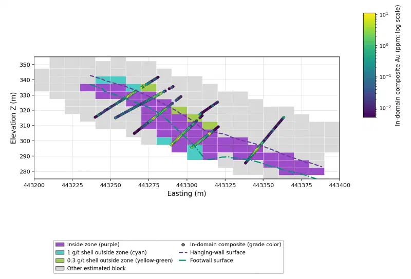
4. Draw zone_section.png at exactly 1800 x 1092 pixels: the same section as shells_section.png (y_index 29 to 31). Colour cells inside the zone purple (HSL 278°, 55%, 55%), 1 g/t shell blocks outside the zone cyan (HSL 177°, 55%, 55%), 0.3 g/t shell blocks outside the zone yellow-green (HSL 79°, 55%, 55%) and other estimated blocks light grey. Draw the interpolated hanging wall and footwall along northing 6,813,885 as two lines, and add the composites as before. No text above the axes and no figure title.
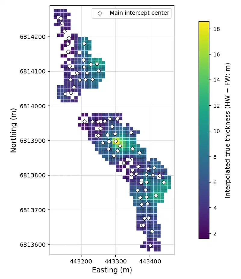
5. Draw zone_thickness.png at exactly 1800 x 1092 pixels: a plan view on equal-scale axes with full coordinates, showing the interpolated true thickness of every 10 m column that holds zone blocks as a filled cell in metres, with the main intercept centres marked and the colour bar right beside the map. No text above the axes and no figure title.

Report only values computed in code in this run. Save the intercept surfaces as CSV (hole_id, along-strike and down-dip centre, hanging-wall and footwall distance, true thickness), the zone flags per block as CSV (x_index, y_index, z_index, in_zone), and every figure as PNG under a new file name.
The agent used 69 of the 73 main intercepts; the other 4 sit more than 20 m from the plane. Their true thickness is 5.4 m at the median and 6.1 m on average, from 1.5 m to 21.7 m. The zone fills 833 blocks, or 416,500 m³.
The two tests give different answers, and the gap is worth seeing:
| Test of the domain composites | Inside the zone | Mean grade | At or above 0.5 g/t | Domain gold inside |
|---|---|---|---|---|
| At each composite’s midpoint | 500 | 2.55 g/t | 83.6% | 82.7% |
| Through the containing block | 515 | 2.15 g/t | 65.6% | 72.2% |
A 5 m high block cannot follow a zone about 6 m thick. So composites at the edges fall into blocks the zone test leaves out, and barren ones fall into blocks it keeps. The surfaces themselves catch 83% of the gold; the blocks keep 72% of it.
Step 4: Export the Zone and the Shells
The last prompt writes the files Geocluster loads: one category table for the voxel wizard, a gram-metre GeoTIFF for the map, and one point per main intercept. In the GeoTIFF, gram-metres are the zone’s true thickness times its grade, so they show where the most gold per square metre of ground sits.
Now the files for Geocluster.

1. Save goanna_zone_voxel.csv for Geocluster's Create voxel with x_index, y_index, z_index and class, one row per block that is in the zone or in a shell. Use class "Gold zone" for zone blocks, "1 g/t shell outside zone" for the other blocks of the 1 g/t shell, and "0.3 g/t shell outside zone" for the remaining blocks of the 0.3 g/t shell. Report the count of each class.
2. Save goanna_zone_gm.tif, a single-band float32 GeoTIFF on the same grid as goanna_idw_column_mean.tif: EPSG:28351, 10 m pixels, 36 columns by 70 rows, transform rasterio.transform.from_origin(443100, 6814280, 10, 10), nodata -9999. For each column with zone blocks, store the gram-metres: the mean interpolated true thickness of the column's zone blocks times the mean au_idw of those blocks. Read it back and report the transform as a, b, c, d, e, f, the bounds, the number of valid pixels and their minimum, maximum and mean. If no raster tool is available, hand this step to the Extended agent.
3. Save goanna_main_intercepts_map.csv with hole_id, east and north (the mean position of the intercept's composites), gram_metres, grade and length_m for each main intercept.

Report only values computed in code in this run. Save every file under the new name given.
The voxel table has 1,162 rows: 833 Gold zone blocks, 51 blocks of the 1 g/t shell and 278 of the 0.3 g/t shell outside the zone. The GeoTIFF has 582 filled cells, from 0.1 to 80.2 gram-metres, with bounds from 443,100 to 443,460 m east and 6,813,580 to 6,814,280 m north. We read those bounds back and checked every cell against the blocks.
The class labels were chosen with care. Geocluster picks each category colour from the label text. So we tested label wordings until the three classes came out purple, cyan and yellow-green, far apart on the colour wheel.
Step 5: Load the Zone and the Shells in 3D
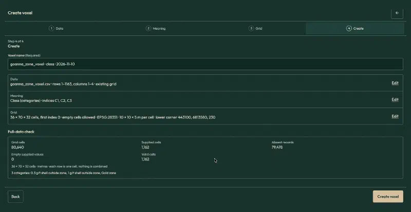
Open goanna_zone_voxel.csv, click Create voxel and fill in the wizard:
| Setting | Value |
|---|---|
| Table meaning | Existing grid |
| Header rows | 1, whole table |
| Value | class, field name Class, Categories |
| Index X, Y, Z | x_index, y_index, z_index |
| Cells along X, Y, Z | 36, 70, 32 |
| First index | 0 |
| Empty cells | Allow empty cells |
| Coordinates | Physical coordinates, metres, Projected CRS |
| CRS | EPSG:28351 |
| Elevation reference | Collar RL, WAMEX A114051 |
| Lower corner X, Y, Z | 443100, 6813580, 230 |
| Cell size X, Y, Z | 10, 10, 5 |
These are the grid settings of the grade voxel from the previous guide, so both voxels line up. Tick the confirmation box on the Meaning page. The full-data check reports 80,640 grid cells, 1,162 supplied and valid, 79,478 absent, and three categories.
Step 6: View and Slice the Zone
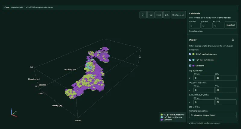
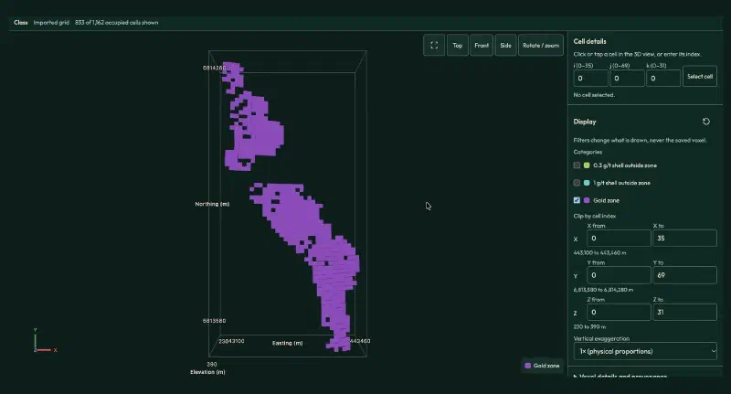
Click Create voxel and open it in 3D. All 1,162 blocks show, with the purple zone wrapped in a thin rim of shell blocks.
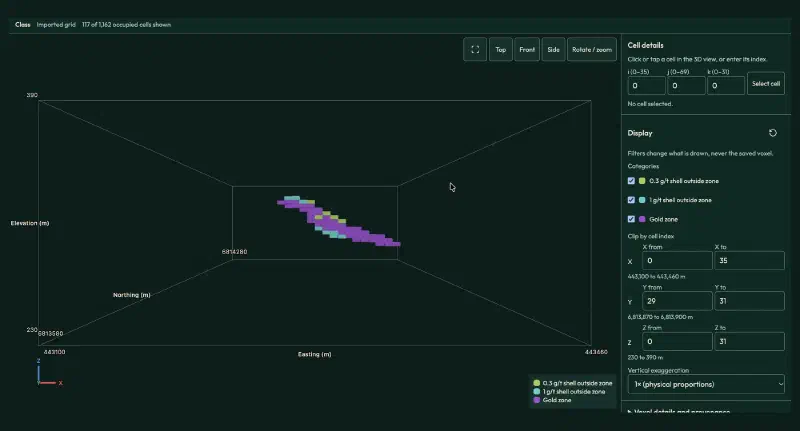
For a slice, set Y from 29 to 31 (northing 6,813,870 to 6,813,900 m) and click Front. This is the section from Step 3, with 117 blocks: 88 in the zone, 15 in the 1 g/t shell and 14 in the 0.3 g/t shell outside it.
Clear the clip, untick the two shell classes under Categories and click Top. The 833 zone blocks form two pods along the trend, the same two pods as the grade maps of the previous guide.
Step 7: Map the Gram-Metres
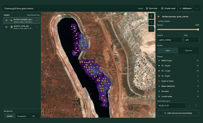
Open Map, click Add layers, choose Grids and images and add goanna_zone_gm.tif, with the Viridis colours. Then open Sample and drillhole tables, click Locate… on goanna_main_intercepts_map.csv and fill in:
- What the rows are: Surface samples, the option for one point per row.
- Sample ID, Assay value, Easting, Northing:
hole_id,gram_metres,east,north. - Qualifier column: leave it empty.
- Coordinate system and Units: GDA94 / MGA zone 51, and
g·m.
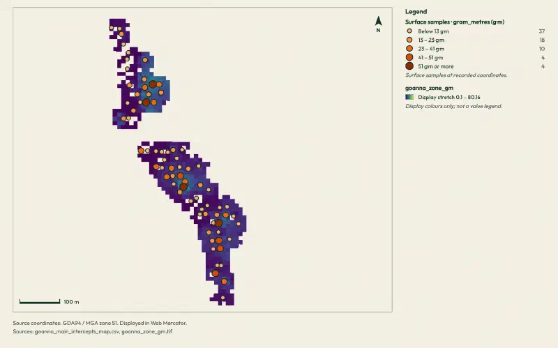
Geocluster splits the 73 intercepts into five classes, from below 13 to 51 gram-metres or more. The points use each intercept’s length along the hole, while the raster uses true thickness, about 10% less here. On the satellite background, the zone runs along the eastern wall of an open pit, like the grade model of the previous guide.
For a clean figure, zoom in on the main map until the zone fills the view. Then click Create visual without Fit to layers, which stops at a fixed zoom.
Grade Shells vs a Mineralized Zone: What the Comparison Shows
Each way to create grade shells gives a different volume for the same gold:
| Outline | Blocks | Volume (m³) | Domain gold inside | Mean grade inside |
|---|---|---|---|---|
| Grade model at 0.3 g/t or more | 1,993 | 996,500 | not tested | not tested |
| 0.3 g/t indicator shell | 894 | 447,000 | 78.6% | 1.83 g/t |
| Zone from intercepts | 833 | 416,500 | 72.2% | 2.15 g/t |
| 1 g/t indicator shell | 288 | 144,000 | 54.2% | 2.98 g/t |
Read together, the steps give a short answer:
- Cutting the smoothed grade model overstates the volume. It keeps more than twice the blocks of the 0.3 g/t shell.
- The zone is the geological answer. It holds a little less gold than the 0.3 g/t shell (72% against 79%) in a slightly smaller volume, at a higher grade. It also matches the 5 m thickness in the report.
- The 1 g/t shell is the rich core. It holds over half the gold in a third of the zone’s volume, and 237 of its 288 blocks lie inside the zone.
- Block size matters. Tested at the composites, the zone holds 83% of the gold; tested through 5 m blocks, only 72%.
Limits When You Create Grade Shells This Way
The result of this workflow carries these limits:
- Rules shape the zone. A 0.5 g/t cut-off, a 2 m minimum and 2 m of internal waste are choices. Other rules give other intercepts and another zone.
- One zone per hole. The zone uses each hole’s main intercept. Smaller intercepts outside it, and 4 main intercepts away from the plane, stay out.
- Simple surfaces. The hanging wall and footwall come from inverse distance between holes, with nothing to stop them thinning to zero or swelling between holes.
- Coarse blocks. The 5 m block height is close to the zone thickness, so the voxel shows the zone only roughly.
- No structural data yet. The archive also holds 410 structure readings from 55 of these holes, 322 of them with raw core angles. They could check the zone’s dip but need a conversion step we left out.
- Volumes, not tonnes. The data has no rock density, and a screening model is not a resource you could report.
- Check the written summary. One report described the plane with the wrong orientation while its numbers were right. Treat the saved tables and figures as the result, and verify historical drilling data against its source. We recomputed every step from the raw WAMEX files.
FAQs
What is a grade shell?
A grade shell is a 3D outline around the rock that is probably above a chosen cut-off grade, such as 1 g/t gold. It comes from assays, not from geology. Geologists use grade shells to see the shape of the rich rock, to plan holes, and to keep later estimates from smearing high grades into barren ground.
What is the difference between a grade shell and a mineralized zone?
A grade shell follows the assays wherever they lead. A mineralized zone is traced from hole to hole, usually with the geology in mind, here as the rich stretch in each hole linked into one body. The two often overlap, but a zone is easier to check against the logs and the reported thickness.
Why not just cut the grade model at the cut-off?
Interpolation smooths grades between holes, so many blocks end up just above the cut-off. In this guide, cutting the inverse distance model at 0.3 g/t kept 1,993 blocks, more than twice the 894 blocks of the indicator shell at the same cut-off. The indicator shell avoids most of that inflation.
What is indicator interpolation?
Indicator interpolation turns each sample into 1 when it is at or above a cut-off and 0 when it is below, then interpolates those values. The result in each block reads as a probability of being above the cut-off. Keeping blocks at 0.5 or more gives a shell; other thresholds give larger or smaller shells.
What are gram-metres?
Gram-metres multiply grade by length, here grams per tonne times metres. Along a hole they use the intercept length, so 10 m at 9.67 g/t is 96.7 gram-metres. On a map they use the zone’s true thickness instead. Either way, one number shows both how rich and how thick the zone is.
How do you choose the cut-off for a grade shell?
Start from what the shell is for. A low cut-off, such as 0.3 g/t here, outlines the whole mineralized system. A higher one, such as 1 g/t, shows the rich core. Compare a few cut-offs against the gold they hold and their volume, and check them against the geology before you choose.
Create Grade Shells in Geocluster
Open the Geocluster web workspace to create grade shells from drillholes in your browser, without writing code or setting up servers. Continue from the grade model of the previous guide, or from your own blocks and composites. Then send the four prompts above and load the zone with the voxel wizard and the map. You get mineralized intercepts, indicator shells at two cut-offs, a linked gold zone and a gram-metre map, each checked against the holes.