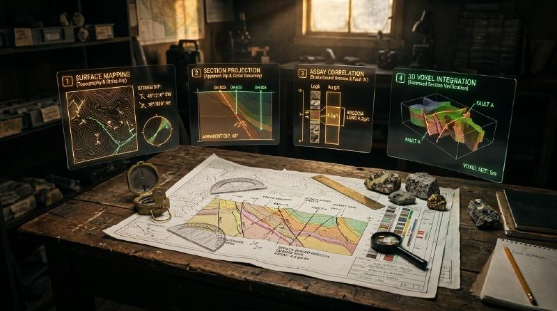
Cross section geology provides a vertical slice through the earth, allowing exploration teams to evaluate structural boundaries and verify subsurface drillhole data.
TL;DR
Looking to master cross section geology and verify exploration measurements against underground rock layers? A geological cross section acts like a vertical slice through the earth, combining surface field mapping with subsurface drillhole data. Consequently, this step-by-step guide explains how to construct balanced sections, project drillholes accurately, and evaluate laboratory assay grades directly against mapped faults and geological contacts.
Key Takeaways
- Cross section geology provides a vertical view of subsurface rock layers and structural boundaries. The open-source GeoCluster research harness provides automated tools for integrating surface maps and drillhole datasets into coherent exploration models.
- A cross section represents an interpretive scientific model rather than an absolute physical measurement. Multiple subsurface geometries can satisfy identical surface field observations and discrete borehole intercepts.
- Vertical exaggeration distorts true planar dips and fault orientations. Interpreters must distinguish visual drawing distortion from underlying coordinate geometry before correlating units across drill traces.
- Assay verification requires projecting samples onto sections within defined distance corridors. Comparing geochemical grades against structural boundaries reveals whether mineralization follows stratigraphic contacts or fault corridors.
What Is Cross Section Geology?
In exploration workflows, cross section geology represents the systematic construction and interpretation of two-dimensional vertical slices through the subsurface earth. Geologists construct each geological cross section by projecting surface structural orientations, stratigraphic contacts, and subsurface borehole data onto a single vertical plane.
Fundamentally, every cross section remains an interpretation rather than an absolute physical measurement. Because direct subsurface observations exist only along discrete drillhole paths, interpreters must infer how strata and structural boundaries connect across unobserved ground.
Therefore, multiple valid cross sections can frequently fit identical surface and drillhole observations. The table below clarifies the primary types of cross sections constructed during exploration programs.
| Cross Section Type | Primary Exploration Scope | Key Validation Principle | Best-Fit Geological Setting |
|---|---|---|---|
| Interpretive Exploration Section | Target generation, drill planning, and assay validation | Consistency with field dips, assays, and mapped contacts | Porphyry, epithermal, and vein-hosted systems |
| Balanced Structural Section | Structural geometry validation and fault displacement testing | Bed-length and cross-sectional area conservation | Contractional fold-and-thrust belts |
| Restored Retro-Deformed Section | Pre-deformation tectonic and basin reconstruction | Kinematic fault restoration and strain reconciliation | Compressional or extensional sedimentary basins |
Specifically, distinguishing routine interpretive sections from formal balanced sections prevents teams from applying strict line-length conservation rules to intrusive or hydrothermally altered settings where those assumptions do not hold.
What Data Goes Into a Cross Section?
Practicing rigorous cross section geology requires compiling diverse observational datasets across varying spatial scales. Furthermore, the quality and resolution of the resulting profile depend directly on the completeness of these primary inputs.
| Primary Data Input | Information Provided | Primary Role in Cross Section |
|---|---|---|
| Topographic Surface Profile | Digital elevation models (DEM) or surveyed station contours | Establishes the upper bounding surface for all contacts and hole collars |
| Geological Surface Map | Lithological units, stratigraphic boundaries, faults, and fold traces | Pins contact locations and fault traces at ground level |
| Structural Measurements | Field strike and dip angles of bedding, foliation, and joints | Defines surface projection vectors and dip directions |
| Drillhole Collar Surveys | Spatial coordinates ($X, Y, Z$) of borehole entry points | Anchors downhole survey traces to the topographic profile |
| Downhole Deviation Surveys | Dip and azimuth measurements recorded at downhole depth intervals | Traces three-dimensional borehole paths through space |
| Lithological Core Logs | Categorical rock descriptions and interval boundaries | Provides discrete subsurface rock intercepts for stratigraphic correlation |
| Analytical Assay Tables | Quantitative element concentrations and sample depth intervals | Supplies geochemical grades to test against interpreted structures |
In complex terrains, geologists also integrate seismic profiles, magnetic inversion depth slices, and ground gravity contours. Consequently, these geophysical layers establish deep structural baselines below the limit of physical drilling.
Teams handling legacy exploration portfolios often extract historical structural contacts from regional archives using geological map processing tools to establish regional baselines.
How to Draw a Geological Cross Section, Step by Step
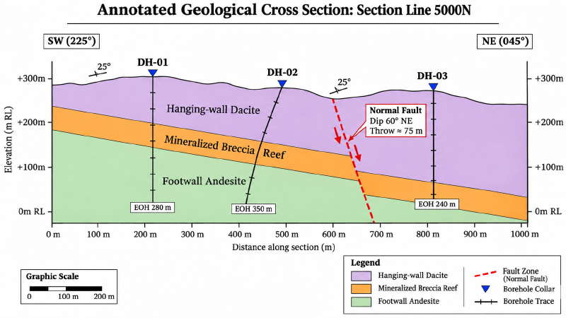
Constructing a section by hand or within computer-aided drafting software follows a rigorous sequence of geometric steps. In practice, adhering to this workflow prevents spatial distortion and minimizes structural contradiction.
Seven-Step Section Construction Workflow
Exploration teams follow a structured progression to convert surface and downhole observations into defensible profiles:
- Step 1: Select the section line orientation. Aligning perpendicular to regional structural strike displays true dips and stratigraphic thicknesses; however, sections are frequently oriented along drill fences, down plunge of mineralized shoots, or across complex fault intersections.
- Step 2: Construct the accurate topographic profile. Transfer elevation contours along the chosen line of section onto profile coordinates.
- Step 3: Plot surface geological contacts and faults. Mark surface intersection points where the section line crosses mapped contacts and faults, accounting for mapping and positional uncertainty.
- Step 4: Calculate and plot apparent dips. If planar structures strike obliquely to the section line, calculate and plot the apparent dip rather than the true field dip.
- Step 5: Plot desurveyed drillhole traces. Apply desurvey calculations to boreholes, project eligible holes onto the section plane within a defined corridor, and mark downhole contact intervals.
- Step 6: Correlate contacts and project structures. Connect corresponding stratigraphic units across boreholes using solid lines for directly observed contacts and dashed lines for inferred boundaries.
- Step 7: Check geometric and structural reasonableness. Verify that layer thicknesses remain geologically plausible and that fault displacements honor the tectonic regime.
Apparent Dip Calculations and Angle Conventions
When a section line crosses dipping planar strata at an oblique angle, the apparent dip visible on the section plane is always shallower than the true dip measured in the field. Plotting true dip on an oblique section artificially distorts bed geometry and leads to incorrect depth predictions.
The relationship between true dip ($\delta$), apparent dip ($\alpha$), and the acute angle between bed strike and the section line ($\beta$) follows trigonometry:
$$\tan(\alpha) = \tan(\delta) \cdot \sin(\beta)$$In this formula, $\delta$ represents true dip ($0^\circ \le \delta \le 90^\circ$), and $\beta$ represents the acute horizontal angle between the strike azimuth of the bed and the section line azimuth ($0^\circ \le \beta \le 90^\circ$). For example, if a bed strikes $045^\circ$ and the section line trends $090^\circ$, the acute angle $\beta$ equals $|090^\circ-045^\circ| = 45^\circ$.
| True Dip ($\delta$) | Strike-to-Section Angle ($\beta$) | Apparent Dip ($\alpha$) on Section | Geometric Consequence |
|---|---|---|---|
| $45^\circ$ | $90^\circ$ (Perpendicular) | $45.0^\circ$ | True dip displayed; $\sin(90^\circ) = 1.0$; no correction required |
| $45^\circ$ | $60^\circ$ | $40.9^\circ$ | Minor apparent flattening; correction required |
| $45^\circ$ | $30^\circ$ | $26.6^\circ$ | Severe flattening; beds appear substantially shallower |
| $45^\circ$ | $0^\circ$ (Parallel to Strike) | $0.0^\circ$ | Complete flattening; $\sin(0^\circ) = 0.0$; beds appear horizontal |
Therefore, exploration geologists calculate apparent dips for every individual orientation station whenever variable fold limbs or oblique fence lines prevent perpendicular alignment.
Vertical Exaggeration Geology and Dip Distortion
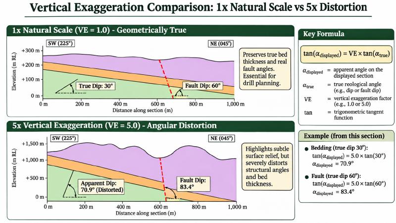
In regional basin studies or environmental investigations, geologists occasionally stretch the vertical scale relative to the horizontal scale. Specifically, this practice, known as vertical exaggeration ($VE$), highlights subtle surface topography and thin near-surface layers:
$$VE = \frac{\text{Vertical Scale}}{\text{Horizontal Scale}}$$For example, a section drawn at a vertical scale of $1:2,500$ and a horizontal scale of $1:5,000$ carries a vertical exaggeration of $2\times$.
However, in exploration geology, vertical exaggeration distorts structural angles on the page. Whenever vertical exaggeration exceeds $1\times$, planar angles steepen artificially on the drawing according to:
$$\tan(\theta_{\text{displayed}}) = VE \cdot \tan(\alpha)$$In practice, interpreters apply a two-step order of operations: first calculate the section apparent dip $\alpha$, then apply vertical exaggeration to determine the displayed angle $\theta_{\text{displayed}}$. Consider a bed with true dip $\delta = 30^\circ$ and strike-to-section angle $\beta = 45^\circ$: its apparent dip $\alpha$ is $22.2^\circ$; drawn at $2\times$ exaggeration, its displayed angle steepens to $39.2^\circ$.
| Section Exaggeration | True Bed Dip ($30^\circ$, $\beta=90^\circ$) | Displayed Angle on Section | Practical Risk to Geologists |
|---|---|---|---|
| $1\times$ (No Exaggeration) | $30.0^\circ$ | $30.0^\circ$ | Preserves true geometric relationships and bed thicknesses |
| $2\times$ | $30.0^\circ$ | $49.1^\circ$ | Steeper appearance; risk of overestimating drilling depth |
| $5\times$ | $30.0^\circ$ | $70.9^\circ$ | Severe distortion; moderately dipping beds appear nearly vertical |
| $10\times$ | $30.0^\circ$ | $80.2^\circ$ | Total loss of structural realism; invalidates protractor checks |
Structural geologists recommend drawing exploration cross sections at an unexaggerated $1:1$ ($1\times$) scale whenever drillhole planning and structural validation represent primary objectives. While vertical exaggeration alters the visual drawing, digital databases maintain true 3D coordinates.
How to Build a Cross Section From Drillhole Data
Integrating drillhole data into cross section geology provides three-dimensional anchors that convert surface geological sketches into validated subsurface models. Moreover, integrating borehole observations requires systematic collar positioning and downhole survey calculation.
Drillhole Desurveying and Spatial Positioning
Technicians convert downhole depth measurements into spatial coordinates using minimum-curvature or balanced-tangential desurveying algorithms. Specifically, balanced-tangential desurveying averages the direction vectors of upper and lower survey stations over half-intervals to calculate three-dimensional trajectories.
The table below provides an illustrative, reproducible drillhole survey setup demonstrating collar coordinates, survey stations, and calculated spatial contact intercepts.
| Survey Station | Depth (m) | Inclination / Dip | Azimuth | Easting ($X$) | Northing ($Y$) | Elevation ($Z$) | Section Offset |
|---|---|---|---|---|---|---|---|
| Collar (DH-04) | $0.0\text{ m}$ | $-60.0^\circ$ | $090.0^\circ$ | $450,210.0\text{ m}$ | $5,400,015.0\text{ m}$ | $+342.0\text{ m}$ | $15.0\text{ m}$ North |
| Contact 1 | $24.5\text{ m}$ | $-59.5^\circ$ | $090.5^\circ$ | $450,222.4\text{ m}$ | $5,400,014.9\text{ m}$ | $+320.8\text{ m}$ | $14.9\text{ m}$ North |
| Breccia Contact | $112.0\text{ m}$ | $-58.0^\circ$ | $091.5^\circ$ | $450,267.8\text{ m}$ | $5,400,013.8\text{ m}$ | $+245.8\text{ m}$ | $13.8\text{ m}$ North |
| Footwall Contact | $118.5\text{ m}$ | $-57.8^\circ$ | $091.6^\circ$ | $450,271.2\text{ m}$ | $5,400,013.7\text{ m}$ | $+240.3\text{ m}$ | $13.7\text{ m}$ North |
| End of Hole | $260.0\text{ m}$ | $-55.0^\circ$ | $092.5^\circ$ | $450,348.5\text{ m}$ | $5,400,010.5\text{ m}$ | $+122.5\text{ m}$ | $10.5\text{ m}$ North |
In this example, the section line is established at Northing $5,400,000\text{ m}$ trending East-West ($090^\circ$). Consequently, the section offset represents the perpendicular distance between the desurveyed borehole position and the section plane.
Contact Intercepts and Uncertainty Display
Next, geologists plot the borehole trace directly onto the section profile. Where boreholes intercept rock units, geologists compare adjacent intercepts across multiple drillholes to delineate unit boundaries.
Following standard geological conventions, draw observed contacts directly supported by drillhole intercepts as solid lines. Conversely, draw inferred continuations through unsampled space as dashed or question-marked lines to communicate uncertainty honestly.
How to Project Data Onto a Cross Section
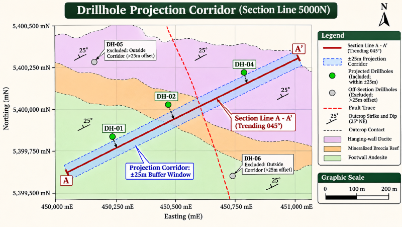
In practical cross section geology, drillholes rarely fall precisely along an idealized two-dimensional section plane. Consequently, geologists must project nearby drillholes, surface outcrops, and geochemical samples onto the section plane within a defined projection corridor.
Projection Corridor Selection Guidelines
Choosing an appropriate projection corridor requires balancing data density against geometric distortion. For example, if the corridor is too narrow, valuable drillhole intercepts are omitted; if the corridor is too wide, along-strike structural changes blur the section.
The table below summarizes illustrative operational guidelines for selecting projection corridor widths across exploration settings.
| Projection Corridor Setting | Selection Criteria | Typical Exploration Scenario | Primary Geometric Risk |
|---|---|---|---|
| Strict ($<10\text{ m}$) | High drill density; steep dips; narrow veins | Infill definition drilling on structural gold veins | Omits valuable step-out holes from adjacent fences |
| Standard ($25\text{ to }50\text{ m}$) | Moderate drill density; uniform strike | Exploration step-out fence drilling | Minor apparent displacement along plunging shoots |
| Broad ($>100\text{ m}$) | Sparse reconnaissance holes; flat strata | Early-stage regional porphyry or basin targeting | Severe distortion if fold hinges plunge or faults terminate |
Geologists display the perpendicular offset distance next to each projected hole collar on the profile. In addition, testing multiple corridor widths ensures that interpreted geometries do not rely on features projected from too far along strike.
Axial Projection in Plunging Structures
When projecting data along plunging fold axes, geologists apply axial projection rather than simple perpendicular projection. In plunging structures, cylindrical fold geometry dictates that subsurface boundaries shift vertically along the fold axis.
Specifically, axial projection adjusts the elevation of projected data points according to the regional plunge:
$$\Delta Z = \Delta L \cdot \tan(\text{plunge})$$Here, $\Delta L$ represents the distance from the borehole to the section plane measured parallel to the fold hinge azimuth. Applying this elevation shift aligns off-section drillhole intercepts with the structural geometry displayed on the section plane.
Teams processing legacy assessment reports can review our guide on how to verify historical drilling data before you use it to ensure collar elevations match topography before projecting historical holes.
How to Compare Samples With Mapped Structures
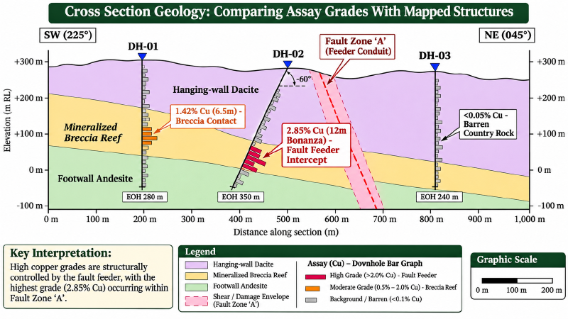
The primary exploration value of cross section geology lies in testing analytical sample measurements against interpreted structural geometry. Plotting geochemical assay grades directly on the cross section reveals the physical controls on mineralization.
For example, plotting copper, gold, or lithium assays along projected drillhole traces highlights whether high-grade intervals cluster along stratigraphic boundaries, fold hinges, or fault damage zones.
Schematic Exploration Cross Section Traverse
The text diagram below depicts an illustrative cross-section traverse across three diamond drillholes testing a mineralized fault and contact system.
===============================================================================
ILLUSTRATIVE SCHEMATIC CROSS SECTION: LINE 5400N (Looking North, 1:1 Scale)
Topography: -----------------\_______________________/-------------------------
Elevation                      [DH-01]            [DH-02]           [DH-03]
+300m                            |                  |                  |
                                 |                  |                  |
+200m     Hanging-wall Dacite    |                  |  Fault Zone 'A'  |
          (Barren: <0.05% Cu)    |                  |  ~~~~~~~~~~~~~~~~|
---------------------------------o 24.5m            |  ~ High Shear  ~ |
+100m                            |                  o 52.0m            |
          Breccia Reef           |                  |  ~ 2.85% Cu    ~ |
          (Mineralized Target)   * [1.42% Cu]       |  ~ (Structural)~ |
---------------------------------o 118.5m           |  ~~~~~~~~~~~~~~~~|
   0m                            |                  o 145.0m           o 18.0m
          Footwall Andesite      |                  |                  |
          (Background: 0.08% Cu) |                  |                  |
-100m                            V EOH 260m         V EOH 280m         V EOH 210m
===============================================================================
Worked Assay Correlation and Geological Hypotheses
Evaluating analytical assay grades against mapped structural positions clarifies deposit architecture and guides step-out drilling. Downhole intervals are represented as discrete sample bars rather than dimensionless points to preserve interval thickness.
The table below summarizes the illustrative drillhole traverse, clearly separating empirical laboratory observations from geological working hypotheses.
| Drillhole ID | From to To (m) | Analyte Grade | Structural / Lithological Position | Empirical Observation | Geological Hypothesis to Test |
|---|---|---|---|---|---|
| DH-01 | $112.0\text{ to }118.5\text{ m}$ | $1.42%\text{ Cu}$ | Contact: Dacite / Breccia boundary | High-grade copper interval coincides with porous breccia reef | Mineralization may be strata-bound; test along-strike permeability |
| DH-01 | $118.5\text{ to }160.0\text{ m}$ | $0.08%\text{ Cu}$ | Footwall Andesite interior | Background copper grades in massive unmineralized volcanic unit | Footwall volcanic sequence represents unmineralized baseline |
| DH-02 | $52.0\text{ to }64.0\text{ m}$ | $2.85%\text{ Cu}$ | Fault Zone ‘A’ sheared zone (dips $65^\circ\text{ W}$) | Elevated copper occurs within intense structural shear corridor | Fault reactivation localized hydrothermal fluid flow; step-out down-dip |
| DH-02 | $64.0\text{ to }145.0\text{ m}$ | $0.04%\text{ Cu}$ | Footwall Andesite sheared zone | Grades drop sharply into unbrecciated footwall wallrock | Mineralization drops sharply away from fault damage envelope |
| DH-03 | $18.0\text{ to }32.5\text{ m}$ | $0.12%\text{ Cu}$ | Hanging-wall Dacite offset contact | Moderate anomalous copper near displaced hanging-wall contact | Fault Zone ‘A’ displacement truncates breccia target horizon |
Geochemical teams investigating multi-element trace signatures can apply geochemical anomaly detection methods to identify subtle pathfinder alteration envelopes flanking these structural conduits.
How to Check a Cross Section Is Reasonable
Because cross sections remain interpretive hypotheses, testing each profile against fundamental cross section geology rules is critical prior to committing exploration capital. Specifically, structural validation relies on four primary consistency tests.
Four Structural Consistency Checks
Interpreters test cross sections against four structural criteria:
- Surface Map Consistency: Depicted contacts, faults, and dips must agree with surface maps within mapping scale, GPS positional uncertainty, and topography constraints.
- Structural Admissibility: Subsurface geometries must represent physically plausible structures for the tectonic regime (for example, consistent normal fault dips in rifts or ramp-flat cutoffs in compressional belts).
- Section Balancing and Retrodeformability: Restoring deformed sedimentary beds back to an undeformed pre-tectonic state must yield continuous beds without unexplained gaps or severe overlaps.
- Stratigraphic Thickness Preservation: Stratigraphic units should maintain reasonable depositional thicknesses unless ductile shearing or fault cutoffs explain localized thinning.
Bed-Length Balancing Tolerances
In contractional fold-and-thrust belts, structural geologists frequently apply line-length balancing diagnostics (Dahlstrom, 1969; Marshak & Mitra, 1988). Under assumptions of plane strain, constant layer thickness, and negligible penetrative strain, bed-length discrepancies between deformed and restored states should generally remain within roughly $5%$ to $10%$.
Discrepancies exceeding this diagnostic range suggest incorrect structural geometry, unrecognized thrust repetitions, or out-of-plane strike-slip displacement. Consequently, interpreters re-evaluate subsurface fault trajectories whenever restored lengths diverge significantly.
Cross Section Software Compared
Modern exploration teams rely on specialized digital tools to construct, validate, and query cross sections from relational databases. Selecting an appropriate tool depends on project scale, structural complexity, and budget constraints.
Software Capability and Workflow Matrix
The table below summarizes leading software platforms across core operational criteria and best-fit exploration workflows.
| Software Platform | Tool Category & Focus | Key Strengths | Critical Operational Limitation | Best-Fit Exploration Workflow |
|---|---|---|---|---|
| QGIS Geoscience Plugin | Open-source GIS extension; 2D section management | Free open-source GIS integration; desurveys drillholes; exports midpoints | Manual contact snapping; 2D only; no native 3D wireframing | Early-stage grassroots GIS mapping and drillhole plotting |
| Seequent Leapfrog Geo | Commercial 3D implicit modeling software | Dynamic 3D cross-section slicers; rapid RBF implicit surface modeling | High proprietary licensing costs; implicit algorithm black-box bias | Advanced deposit modeling and resource estimation |
| Datamine Discover | Commercial CAD drafting & mapping platform | Comprehensive 2D presentation cartography; downhole strip log rendering | Desktop-bound license; steep learning curve for junior geologists | Mining production cartography and statutory compliance logs |
| GeoCluster Research Harness | Open-source research harness; tabular data ingestion | Automated table extraction; coordinate parsing; auditable evidence links | Does not auto-pick structures or replace manual logging | Open-source data preparation and audit pipelines |
Teams evaluating enterprise solutions can consult our guide on geological data management software to compare database structures and audit trails across commercial logging platforms.
Cross Sections and 3D Models
Cross sections and three-dimensional block models represent complementary views of a subsurface geological interpretation. Rather than competing approaches, a cross section provides a constrained planar slice through a volumetric three-dimensional model.
In modern implicit modeling engines, geologists utilize cross sections as interactive drawing canvases. Interpreters sketch guide planes and fault polylines on section slices, and the modeling engine interpolates continuous 3D surfaces through Radial Basis Functions (RBF) or discrete meshes.
Furthermore, when teams construct discrete block or voxel grids, cross sections provide essential quality assurance. Geologists slice through block models along historical exploration lines to verify that interpolated grade boundaries honor mapped structural contacts.
Teams interested in volumetric modeling workflows can explore how continuous surfaces are discretized into cellular representations on the 3D voxel model demo.
FAQs
What is a cross section in geology?
A geological cross section represents an interpretive vertical profile illustrating subsurface rock arrangements and structural geometry across an exploration project. It integrates surface field mapping, structural strike-and-dip readings, and desurveyed drillhole intervals onto a 2D plane to depict underground stratigraphic contacts, fault offsets, and folded rock layers.
How do you draw a geological cross section?
To draw an accurate geological cross section, geologists establish a profile line across the target, construct a topographic profile, and plot surface contact points. Next, they calculate apparent dips, project desurveyed drillholes within a defined corridor, correlate stratigraphic intervals between boreholes, and check geometries for structural consistency.
What is vertical exaggeration and why does it matter?
Vertical exaggeration represents the ratio of vertical scale to horizontal scale on a cross section drawing. While exaggerating vertical scale highlights subtle surface topography and thin horizontal strata, it artificially steepens planar bed dips, distorts structural fault angles, and invalidates direct geometric protractor measurements on the page.
What data do you need for a cross section?
Constructing an auditable cross section requires a digital elevation profile, surface geological maps with structural strike and dip measurements, and verified drillhole collar coordinates. Furthermore, interpreters integrate downhole deviation surveys, lithological core descriptions, analytical geochemical assay tables, and deep geophysical baselines such as seismic or gravity inversion profiles.
How do you project drillholes onto a cross section?
Geologists establish a defined projection corridor around the profile line, calculating perpendicular or axial offset distances for nearby boreholes. In addition, only drillhole intervals falling within the selected corridor width are projected onto the section plane, with offset distances and downhole interval lengths displayed clearly on the drawing.
What is a balanced cross section?
A balanced cross section represents a structural interpretation through deformed terrain that can be restored geometrically to an undeformed pre-tectonic state without unexplained volume changes or bed-length gaps. This validation technique applies primarily to contractional fold-and-thrust belts and extensional fault systems under line-length and area-conservation rules.
Can software draw a cross section for me?
Exploration software packages automate topographic slicing, borehole desurveying, interval rendering, and projection buffering across relational drillhole databases. However, connecting complex structural contacts between drillhole intercepts, evaluating fault kinematics, and selecting valid geological interpretations requires manual synthesis and critical field validation by experienced exploration geologists.
Try It With Geocluster
The open-source GeoCluster research harness provides automated tools and agent workflows for reading exploration documents, desurveying drillholes, and structuring historical datasets.
Read our practical guide on how to verify historical drilling data before you use it to validate collars, surveys, and assays before updating your exploration database.