
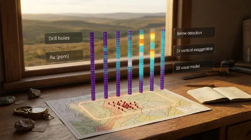
TL;DR: Want to see what your drill holes found, depth by depth, without writing code? Drill hole visualization draws each hole where it was drilled and colours it by what the lab measured. In the Geocluster workspace you join hole locations to lab results, bin them into a 3D grid and slice it, or ask the built-in AI agent for a 2D view along a line. Nothing is guessed between holes, so this is the first step toward a geological cross section, not the cross section itself. Lab results too small to measure are counted and left out, never turned into zeros. We show every step on Wattle Creek, a free synthetic drilling dataset.
What Is Drill Hole Visualization?
Drill hole visualization shows the measured data along each drill hole, such as gold in parts per million (ppm), at its true position and depth. It is the first stage of geological modelling and estimation: you look at what the holes found before deciding how the ground between them connects.
A geological cross section goes further. It fills the ground between holes by interpolation or interpretation, and the final version often hides the holes altogether. A drill section sits in between: interpolated geology with the holes still drawn on top.
This guide, part 1 of a series, covers only the first stage. Every view below shows measured intervals and leaves unsampled ground empty. Later parts move on to inclined holes with rock types, and then to interpolation.
Drill Hole Data Used in This Guide
Wattle Creek is a synthetic dataset released into the CC0 public domain. Because the sample has no lithology table and its collar elevations are invented, treat it as a demonstration rather than a real deposit.
The files ship in the open-source Geocluster research harness under runtime/demo-bundles/wattle-creek/v1. Upload drilling/collars.csv and drilling/assays.csv to a Geocluster project to follow along.
- 140 vertical holes and 3,152 assay intervals of 5 m each, with gold (
au_ppm) and copper (cu_ppm). Coordinates are in EPSG:7851 (GDA2020 MGA zone 51), in metres. - Hole WC141 has results but no location. It matters in step 1.
- 120 gold results are below detection, written as
<0.01or<0.005. - The collar elevation
rlis invented, with no surveyed datum.
How Do I Visualize Drill Hole Data in Geocluster?
There are two routes. The 3D route bins the intervals into a grid you can slice in any direction. The 2D route asks the agent for one figure along a line you choose.
Step 1: Join Drill Hole Collars to Assays
The 3D model needs locations and results in one table. Open the agent, attach assays.csv and collars.csv with @, and paste this prompt:
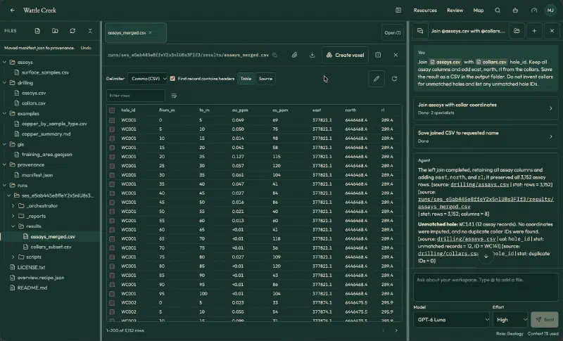
Join assays.csv with collars.csv by hole_id. Keep all assay columns and add east, north, rl from the collars. Save the result as a CSV in the output folder. Do not invent collars for unmatched holes and list any unmatched hole IDs.The agent reported a left join that kept all 3,152 rows. It listed WC141 (12 intervals) as unmatched and did not invent coordinates. Open the saved assays_merged.csv and tick First record contains headers. Otherwise, the header row counts as data (3,153 rows) and columns show as Column 2, Column 3.
Step 2: Build the 3D Voxel Model
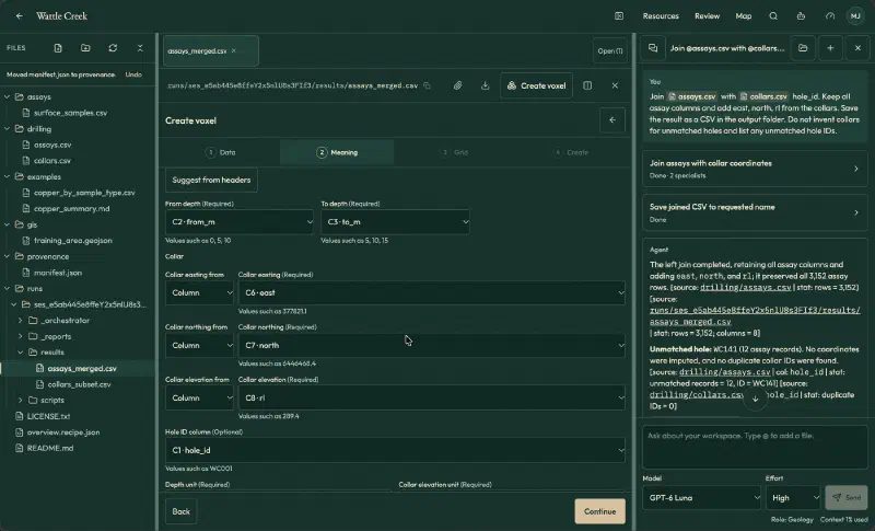
A voxel is a 3D cell, like a pixel in 3D. Click Create voxel. The wizard has four steps: Data, Meaning, Grid and Create. Use these settings:
| Setting | Value |
|---|---|
| Table meaning | Observations |
| Header rows | 1 |
| Geometry | Vertical intervals |
| From depth, To depth | from_m, to_m |
| Collar easting, northing, elevation | east, north, rl (all as columns) |
| Hole ID | hole_id |
| Coordinates | Projected CRS, EPSG:7851, metres |
| Elevation reference | Invented collar RL, no surveyed datum |
| Value | au_ppm, name Au, numbers, unit ppm |
| Cell size | 10 × 10 × 5 m (the wizard’s suggestion) |
| Value per cell | Length-weighted mean |
| Censored values | Exclude and count |
The Suggest from headers button fills most columns for you. Confirm each one.
Step 4 runs a full-data check before anything is saved. It read 3,152 rows and accepted 3,020. The other 132 were left out: 120 below detection and 12 without coordinates (WC141). The grid is 72 × 195 × 32 cells (449,280 in total), and 3,193 hold data.
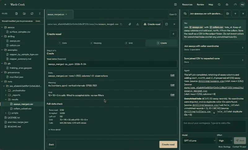
Click Create voxel, wait for the four stages to finish, then click Open in 3D.
Step 3: Slice the 3D Drill Hole Model
The viewer has three groups of controls:
- Clip by cell index: X, Y and Z from/to boxes. The metres each range covers appear below the boxes.
- Top, Front and Side camera buttons.
- Display options: vertical exaggeration (1x to 10x), colour scale (fit to shown cells, full range or logarithmic) and a grade filter.
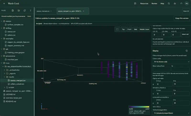
For an east-west slice, set Y from 0 to 8 (northing 6,446,460 to 6,446,550 m) and click Front. It shows 169 cells and seven holes, with empty ground between them.
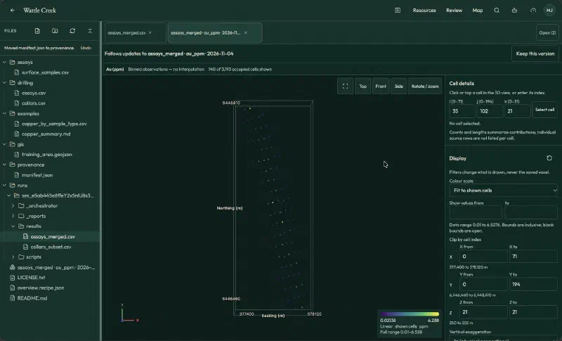
For a level map, set Z from and Z to both to 21 (250 to 255 m elevation) and click Top. You get 140 cells, one per hole.
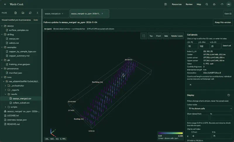
Finally, click a cell to check it. Cell (35, 102, 21) shows 5.991 ppm from two rows over 5 m. By hand, hole WC074 has 7.20 ppm over 3.7 m of the cell and 2.55 ppm over 1.3 m: (3.7 × 7.20 + 1.3 × 2.55) / 5 = 5.991.
Step 4: Draw a 2D Drill Hole View With the Agent
For one flat figure along a line, ask the agent. This is the prompt we used:
Using assays_merged.csv (hole_id, from_m, to_m, au_ppm, cu_ppm, east, north, rl), draw a vertical cross section along the straight line through collars WC001 and WC007, including holes within 25 m of that line. Place each hole at its distance along the line, draw each assay interval as a coloured strip from collar elevation (rl minus depth), and colour by Au (ppm). Show <DL intervals in a separate neutral colour, not as zero. Use 2x vertical exaggeration, add a legend, scale, and axis labels with units. Save a PNG in the output folder. List the holes used, the distance of each from the line, and any assumptions. Leave WC141 out. Do not invent data.The agent used seven holes along the 306.6 m line. The furthest, WC002, sits 5.9 m off it. It used 168 intervals: 161 numeric gold values (0.013 to 3.46 ppm) and seven below detection, all in WC001 and drawn in grey. We recomputed these counts from the table and they match.
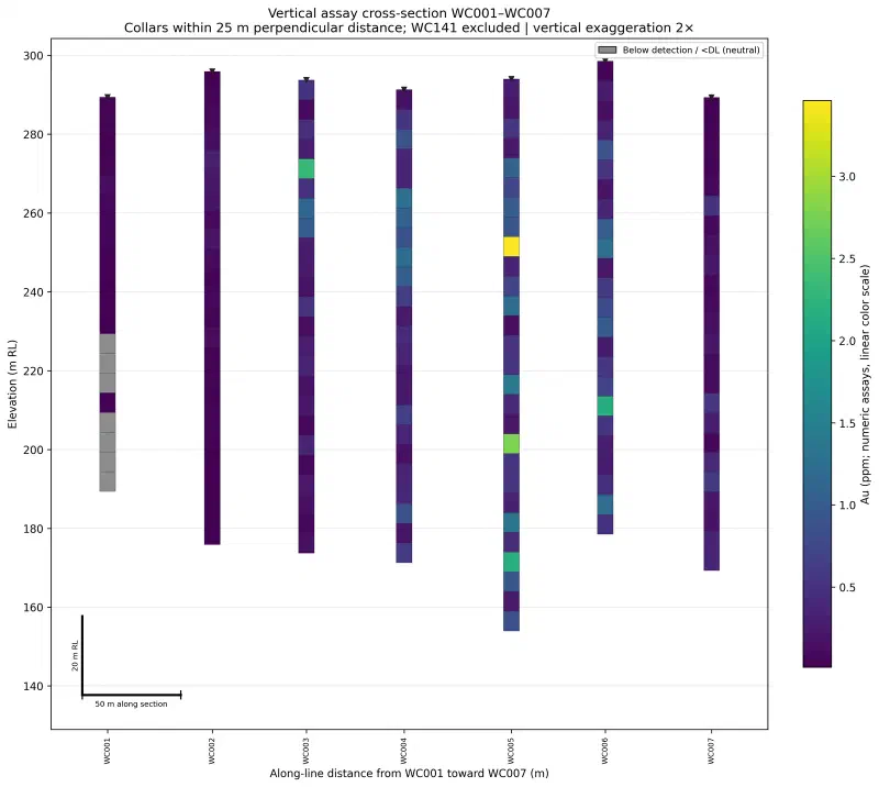
The two routes complement each other. For example, the 2D view shows each 5 m interval at its own value, while the voxel model averages intervals that straddle a cell boundary. As a result, its highest cell (6.528 ppm) is below the highest interval (7.37 ppm).
Limits of This Drill Hole Visualization
- Not a cross section yet. Nothing is interpolated or interpreted between holes, so these views cannot show how ore zones or rock units connect.
- No rock types. The sample has no lithology table, so every view shows grade only.
- Vertical holes only. The wizard setting used here treats every hole as vertical.
- Perspective and legends. Front and Side views use perspective, so do not measure distances on them. With Fit to shown cells, the legend rescales each time you clip.
- Below-detection results are not zeros. Assay detection limits vary by lab, so we leave censored values out instead of substituting a number.
FAQs
What does drill hole visualization show?
Drill hole visualization shows measured data, such as assay grades, along each drill hole at its true position and depth. It displays only what the holes sampled and leaves the ground between them empty. Geologists use it first, to check the data and spot patterns before interpolating or interpreting anything.
How is drill hole visualization different from a geological cross section?
Drill hole visualization shows only measured intervals along each hole. A geological cross section fills the ground between holes by interpolation or interpretation, and often hides the holes in the final figure. A drill section sits in between, showing interpolated geology with the drill holes still drawn on top.
Why must collar locations and assays be in the same table?
Geocluster’s Vertical intervals builder reads each interval’s collar coordinates, depth range and assay value from a single row. If your collars and lab results sit in separate CSV files, join them by hole ID first. Unmatched holes such as WC141 are counted and excluded rather than given invented coordinates.
What happens to assay results below the detection limit?
Results below the lab detection limit are excluded from numeric calculations and counted separately, so no fake zero or half-limit number enters the model. In the 2D view, the AI agent plots censored intervals in neutral grey. That prevents differing lab limits from creating false grade patterns across holes.
Does a drill hole voxel model estimate grades between holes?
No, an observation voxel model fills only the 3D cells that drill holes physically intersect and leaves unsampled ground empty. In the Wattle Creek example, just 3,193 of 449,280 cells contain data. Turning sparse drill intercepts into a resource estimate requires geological domaining and spatial interpolation.
Why use vertical exaggeration on a drill hole view?
Vertical exaggeration stretches the depth axis relative to horizontal distance, so thin assay intervals stay readable across wide drill spacing. For example, a 2x setting doubles apparent vertical thickness along a 300 m line. Always state the exaggeration factor on the figure, because stretching steepens apparent dips.
Visualize Drill Hole Data in Geocluster
Open the Geocluster web workspace to visualize drill hole data in your browser without writing code or setting up servers. Next, create a project, upload the Wattle Creek collars.csv and assays.csv files (or your own drill hole tables), and repeat the steps above to slice a 3D voxel model or draw a 2D view.