Key Takeaways
- The task today: Exploration geologists must identify every geochemical anomaly in soil, rock chip, and drillhole assay tables. Exploration teams routinely use statistical calculations in desktop software to distinguish subtle mineralisation signatures from barren regional background.
- The problem: Parametric methods like z-score assume normal distributions and fail when skewed populations or extreme outliers distort sample means. In contrast, rigid thresholding flags false positives from regolith variations or misinterprets below-detection analytical noise as genuine exploration targets.
- What the tool does: GeoCluster is a browser-based AI agent for geological data analysis, available in open-source and Enterprise editions. It compares anomaly rankings across z-score, median absolute deviation, and background-ratio models while preserving complete evidence traceability back to laboratory certificates.
TL;DR
A geochemical anomaly represents an elemental concentration that significantly departs from expected barren background values, indicating potential mineralisation, weathering enrichment, or contamination. Standard parametric methods like mean plus two standard deviations (z-score) assume a normal distribution, making them vulnerable to skewness and outlier masking in multi-element datasets. Robust non-parametric alternatives such as median absolute deviation (MAD) and local background ratios resist extreme values and provide reliable thresholding when anomalies constitute less than ten percent of samples. By validating statistical outliers against geological domains, regolith context, and below-detection assay flags, exploration teams prioritize defensible drilling targets.
What is a geochemical anomaly?
A geochemical anomaly is an elemental concentration that departs significantly from normal ambient background concentrations in surrounding barren rocks. Specifically, it marks an unusual geochemical deviation caused by hydrothermal mineralisation, secondary regolith scavenging, environmental contamination, or analytical error. In exploration geology, identifying an anomaly provides an essential vector toward concealed mineral deposits.
To prevent misinterpreting raw numbers, exploration teams separate four distinct concepts:
- Statistical Outlier: An extreme numerical value flagged by a mathematical formula or percentile cutoff.
- Geochemical Anomaly: A significant departure from ambient background concentrations in a given geological domain.
- Exploration Target: A candidate area integrating geochemical anomalies with structural, geophysical, and geological mapping.
- Mineralised Target: A geologically validated zone confirmed by diamond drilling to contain economic mineralisation and continuity.
According to CRC LEME exploration guidelines, geochemists distinguish three core baseline terms:
- Background: The natural, ambient elemental abundance across barren host rocks.
- Threshold: The statistical boundary line separating normal background from anomalous concentrations.
- Anomaly: Any measured concentration exceeding the established threshold cut-off.
Geochemical background and threshold: how do you set them?
Setting a geochemical threshold requires practical geological judgement rather than applying a rigid formula. In early exploration programmes, geologists often applied arbitrary multipliers or fixed percentile cut-offs. However, elemental abundance varies dramatically across differing lithologies. For example, a nickel concentration of 200 ppm is highly anomalous in granite, yet falls well within barren background for ultramafic komatiite.
Furthermore, setting thresholds requires careful treatment of censored analytical data. Testing laboratories report below-detection measurements as inequality strings, such as “<0.01 ppm”. Replacing these below-detection values carelessly with arbitrary constants or zeros can bias calculated means and inflate standard deviations, distorting subsequent threshold calculations. While substituting half the analytical detection limit is an accepted operational convenience for preliminary spatial mapping, heavily censored datasets (>15% below detection) require specialized methods such as Kaplan-Meier survival analysis or regression on order statistics.
Consequently, geologists must inspect how their database manages each analytical detection limit before running statistical calculations. Proper handling ensures that low-level analytical noise does not distort regional background baselines.
z-score anomaly detection: mean plus or minus two standard deviations
The classic statistical approach to geochemical anomaly detection relies on parametric z-scores. Geochemists calculate both a standardized z-score metric (z = (x - mean) / SD) and a threshold cut-off in original measurement units. Geochemists commonly calculate this threshold as the sample mean plus two standard deviations (mean + 2 SD). Under a theoretical Gaussian normal distribution, roughly 97.7% of samples fall below this limit. Therefore, approximately 2.3% of the upper tail is flagged as anomalous.
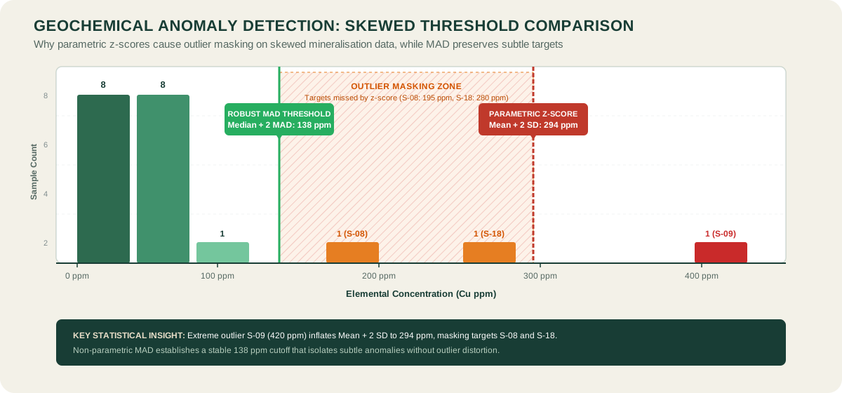
In practice, the classic z-score anomaly method breaks down when applied to raw geochemical assays. Elemental concentrations in mineralised districts typically follow positively skewed log-normal or multi-modal distributions. High-grade outlier samples strongly inflate both the arithmetic mean and the standard deviation.
Consequently, extreme values shift the threshold upward, causing an issue known as outlier masking. As a result, subtle but economically significant mineralisation halos fail to trigger the statistical threshold. Applying a logarithmic transformation prior to calculating z-scores partially mitigates positive skewness. However, log transformations cannot resolve multi-modal distributions caused by mixed rock types.
Median absolute deviation geochemistry: robust anomaly detection
The median absolute deviation (MAD) provides a non-parametric, outlier-resistant alternative to standard deviation. Unlike the arithmetic mean, the sample median remains unaffected by extreme outlier values. The median absolute deviation geochemistry calculation measures the median of absolute deviations from the sample median:
MAD = median(|x_i - median(x)|)
To construct an anomaly threshold comparable to standard deviations, geochemists multiply the raw MAD by a scale factor of 1.4826 to achieve asymptotic consistency with normal distributions. They define the robust threshold as the median plus two scaled MAD units (median + 2 MAD), while evaluating individual sample departures through a robust score ((x - median) / scaled_MAD). As demonstrated by CRC LEME studies, median + 2 MAD provides superior stability against skewness. Specifically, it works reliably when anomalous samples represent up to 10% of the total dataset.
Furthermore, MAD resists outlier masking because extreme high-grade samples cannot distort the median baseline. Consequently, exploration teams identify subtle, low-contrast geochemical halos that parametric tests miss completely.
Background ratio for geochemical anomaly detection
The background-ratio method evaluates elemental concentrations relative to a designated local or lithological background baseline. Rather than calculating a global threshold across an entire regional survey, this approach normalises each sample against its specific geological domain:
Background Ratio = Sample Concentration / Local Background Median
A background ratio of 1.0 represents typical barren background. In contrast, ratios exceeding 3.0 or 5.0 highlight localized enrichment factors. This approach prevents lithological bias across district-scale surveys. Specifically, it ensures that low-contrast anomalies in unreactive rocks receive equal scrutiny as high-contrast signatures in reactive lithologies.
Geochemical anomaly detection methods compared: z-score, MAD and ratio
| Evaluation Dimension | z-score (Mean + 2 SD) | Median Absolute Deviation (MAD) | Background Ratio |
|---|---|---|---|
| Statistical Model | Parametric | Non-parametric, resistant | Relative normalisation |
| Distribution Assumption | Strict Gaussian normality | Symmetric core distribution | Domain-specific median |
| Outlier Sensitivity | High (mean and SD inflated) | Low (resists extreme tail) | Low (median baseline protected) |
| Best Exploration Fit | Homogeneous single-lithology tables | Regional tables with <10% outliers | Multi-lithology mapped districts |
| Primary Failure Mode | Outlier masking of subtle targets | Over-flags dispersed multi-phase data | Requires accurate domain mapping |
A worked example with the same dataset
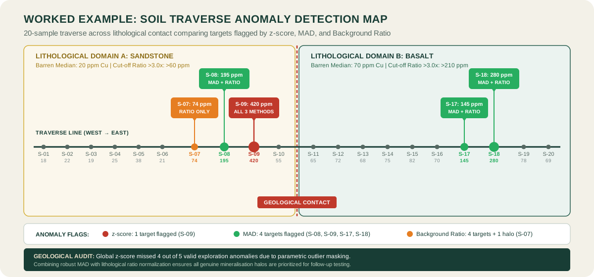
To compare operational differences between methods, consider a 20-sample soil geochemical traverse across a lithological contact between sandstone and basalt. The dataset presents copper concentrations in parts per million (cu_ppm). All values in the following demonstration table are mathematically audited across all three methods.
| Sample ID | Lithology | Cu (ppm) | z-score (SD units) | Robust MAD Score | Background Ratio | Anomaly Classification |
|---|---|---|---|---|---|---|
| S-01 | Sandstone | 18 | -0.77 (Normal) | -1.51 (Normal) | 0.90 (Normal) | Barren background |
| S-02 | Sandstone | 22 | -0.73 (Normal) | -1.39 (Normal) | 1.10 (Normal) | Barren background |
| S-03 | Sandstone | 19 | -0.76 (Normal) | -1.48 (Normal) | 0.95 (Normal) | Barren background |
| S-04 | Sandstone | 25 | -0.70 (Normal) | -1.30 (Normal) | 1.25 (Normal) | Barren background |
| S-05 | Sandstone | 38 | -0.57 (Normal) | -0.92 (Normal) | 1.90 (Normal) | Weakly elevated |
| S-06 | Sandstone | 21 | -0.74 (Normal) | -1.42 (Normal) | 1.05 (Normal) | Barren background |
| S-07 | Sandstone | 74 | -0.21 (Normal) | +0.13 (Normal) | 3.70 (Flagged) | Subtle halo (Ratio only) |
| S-08 | Sandstone | 195 | +1.01 (Normal) | +3.68 (Flagged) | 9.75 (Flagged) | Anomalous (MAD + Ratio) |
| S-09 | Sandstone | 420 | +3.26 (Flagged) | +10.28 (Flagged) | 21.00 (Flagged) | High-grade (Unanimous) |
| S-10 | Sandstone | 55 | -0.40 (Normal) | -0.43 (Normal) | 2.75 (Normal) | Elevated halo |
| S-11 | Basalt | 65 | -0.30 (Normal) | -0.13 (Normal) | 0.93 (Normal) | Barren background |
| S-12 | Basalt | 72 | -0.23 (Normal) | +0.07 (Normal) | 1.03 (Normal) | Barren background |
| S-13 | Basalt | 68 | -0.27 (Normal) | -0.04 (Normal) | 0.97 (Normal) | Barren background |
| S-14 | Basalt | 75 | -0.20 (Normal) | +0.16 (Normal) | 1.07 (Normal) | Barren background |
| S-15 | Basalt | 82 | -0.13 (Normal) | +0.37 (Normal) | 1.17 (Normal) | Barren background |
| S-16 | Basalt | 70 | -0.25 (Normal) | +0.01 (Normal) | 1.00 (Normal) | Barren background |
| S-17 | Basalt | 145 | +0.51 (Normal) | +2.21 (Flagged) | 2.07 (Elevated) | Anomalous (MAD + Ratio) |
| S-18 | Basalt | 280 | +1.86 (Normal) | +6.17 (Flagged) | 4.00 (Flagged) | High-grade (MAD + Ratio) |
| S-19 | Basalt | 78 | -0.17 (Normal) | +0.25 (Normal) | 1.11 (Normal) | Barren background |
| S-20 | Basalt | 69 | -0.26 (Normal) | -0.01 (Normal) | 0.99 (Normal) | Barren background |
Interpreting geochemical anomaly results across the dataset
Across the 20 samples, the arithmetic mean is 94.5 ppm with a sample standard deviation (ddof=1) of 99.8 ppm. The parametric mean + 2 SD threshold equals 294.2 ppm. Consequently, the classic z-score cutoff flags only one extreme sample (S-09 at 420 ppm). Because S-09 severely inflates the standard deviation, parametric thresholding completely masks moderate mineralisation signatures such as S-08 (195 ppm) and S-18 (280 ppm).
In contrast, the global median across all 20 samples is 69.5 ppm with a raw MAD of 23.0 ppm. Multiplying by 1.4826 yields a scaled MAD of 34.1 ppm, producing a non-parametric threshold (median + 2 scaled MAD) of 137.7 ppm. Consequently, the MAD method successfully flags S-08, S-09, S-17, and S-18 without suffering from extreme outlier masking. However, calculating a single global MAD threshold across mixed rock types fails to flag S-07 (74 ppm). In sandstone, where typical background is 20 ppm, 74 ppm represents a significant 3.7-fold enrichment that a global threshold overlooks.
Meanwhile, the background-ratio method normalises samples by lithological domain. Calculating baseline medians from unmineralized samples yields 20 ppm for sandstone and 70 ppm for basalt. Normalising concentrations against these baselines cleanly isolates candidate exploration anomalies: S-07 (ratio 3.70), S-08 (ratio 9.75), S-09 (ratio 21.00), and S-18 (ratio 4.00). Barren basalt samples (65 to 82 ppm, ratios 0.93 to 1.17) remain correctly classified as normal background.
How to check a geochemical anomaly before you rank targets
Statistical thresholding represents only the initial filter in geochemical anomaly detection. Before exploration capital is allocated to diamond drilling, geologists must validate statistical outliers against spatial and geological reality.
Spatial pattern and halo coherence
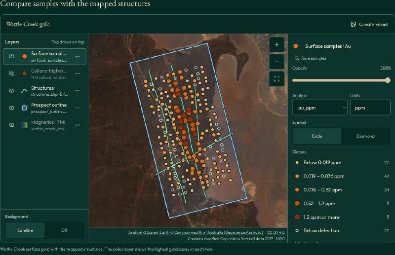
First, check spatial coherence across sampling grids. An isolated high-grade sample surrounded by barren neighbours often reflects analytical contamination, coarse nugget effects, or clerical error. In contrast, a cluster of contiguous elevated values crossing multiple sample lines provides evidence of a dispersed geochemical dispersion halo.
Regolith context and scavenger phases
Second, evaluate regolith context and scavenger phases. In weathered terrains, secondary manganese and iron oxyhydroxides strongly scavenge transition metals, creating pseudo-anomalies that do not reflect bedrock mineralisation. Field teams can deploy portable core scanning and XRF tools to collect real-time multi-element data, allowing geologists to normalise pathfinder metals against iron and manganese scavengers.
Multi-element pathfinder associations
Third, verify multi-element associations. A porphyry copper signature typically exhibits coupled elevation across molybdenum (mo_ppm), gold (au_ppm), and arsenic, whereas isolated copper spikes frequently represent cultural contamination or lithological variation. Future workflows will incorporate automated geochemical data clustering to recognise multivariate element associations across regional datasets.
Finally, autonomous workflows using a specialized geology AI agent allow geologists to cross-examine spatial anomaly clusters against historical structural maps, verifying that candidate targets align with regional fault architectures.
Geochemical anomaly detection in software
Modern exploration workflows integrate statistical anomaly detection directly into exploration software platforms. Exploration teams use dedicated geochemical data analysis software to automate the calculation of z_score metrics, non-parametric MAD values, and lithological background ratios across multi-element datasets.
Furthermore, teams deploy specialised geochemical clustering and anomaly tools to map multivariate signatures and filter false positives from regolith scavenging.
Evaluating these capabilities helps geologists identify the best geological data analysis software for their exploration programmes. By computing multiple statistical thresholds simultaneously, modern software allows exploration teams to identify subtle low-contrast signatures that single parametric tests overlook. In addition, automated platforms preserve complete audit trails linking calculated anomaly scores directly to primary laboratory certificates.
FAQs
What does a geochemical anomaly indicate in mineral exploration?
A geochemical anomaly indicates an elemental concentration that significantly exceeds local background levels. In mineral exploration, it suggests the presence of hydrothermal mineralisation, structural fluid pathways, or secondary weathering enrichment, providing a primary indicator for target drill testing.
How do you set a geochemical threshold?
You set a geochemical threshold by evaluating statistical distributions alongside geological domains. Exploration teams use statistical methods such as median plus two median absolute deviations (MAD) or local background ratios, validating calculated cut-offs against known barren lithologies.
What is the difference between z-score and MAD?
The z-score method calculates thresholds using parametric mean and standard deviation, making it vulnerable to distortion from extreme outliers. In contrast, median absolute deviation (MAD) uses non-parametric medians, providing an outlier-resistant threshold that avoids masking subtle anomalies.
Why is mean plus two standard deviations not always reliable?
Mean plus two standard deviations assumes a normal Gaussian distribution. However, geochemical data are typically positively skewed and multi-modal. Extreme high-grade values inflate the mean and standard deviation, artificially elevating the threshold and masking genuine low-contrast mineralisation.
Do I need to log-transform geochemical data first?
Logarithmic transformations help reduce positive skewness in single-population log-normal datasets. However, log transforms cannot separate mixed geological populations or multi-modal distributions. For complex regional tables, robust non-parametric methods like MAD or background ratios perform more reliably.
How do below-detection values affect anomaly detection?
Below-detection values introduce left-censored data into assay tables. Substituting arbitrary values or zeros can distort calculated means and standard deviations, shifting statistical thresholds. Proper handling requires substituting half the detection limit while preserving raw data flags.
How do I know if an anomaly is real?
You verify an anomaly by checking spatial clustering, regolith context, and multi-element associations. A genuine anomaly typically forms a coherent multi-sample spatial cluster with supporting pathfinder elements, rather than an isolated single-point spike.
Try It With Geocluster
GeoCluster is a browser-based AI agent designed for exploration geologists who require robust geochemical anomaly detection and reliable evidence traceability. Available in open-source and Enterprise editions, GeoCluster connects directly to geological assay tables to automate statistical exploration workflows.
The platform calculates parametric z-scores, robust median absolute deviations, and domain-specific background ratios simultaneously. It treats below-detection assays as half the analytical limit while preserving visible quality flags, composites drillhole intervals with length-weighted means, and maintains strict evidence traceability linking every ranked anomaly back to its primary laboratory certificate. Explore the open-source codebase on the GeoCluster research harness repository to deploy audit-ready anomaly detection across your exploration projects.