TL;DR
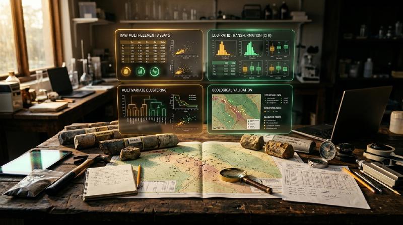
Looking to group exploration rock and soil samples by their chemistry without manual sorting? Geochemical data clustering uses automated pattern-matching algorithms to group samples that share similar element concentrations. Consequently, this guide compares K-means, DBSCAN, and PCA, showing how to prepare laboratory assay data, select appropriate parameters, and confirm that mathematical groups match real geology.
Key Takeaways
- Geochemical data clustering groups exploration assay samples by shared chemistry without requiring manual labels. The open-source GeoCluster research harness provides automated tools and clustering algorithms for evaluating multi-element geochemical surveys.
- Different clustering algorithms assume distinct geometric shapes in data. K-means forces all samples into round clusters of similar size, whereas DBSCAN traces irregular paths and separates unassigned density outliers.
- Principal component analysis simplifies dozens of measured elements into combined factors but does not form clusters on its own. Exploration geologists use it before clustering to identify connected element groups and reduce dataset dimensions.
- Statistical clusters require field verification and geological mapping to confirm they represent real rock types or alteration. A mathematical grouping that contradicts mapped lithology is an artifact of the calculation, not an undiscovered deposit.
Applying geochemical data clustering enables mineral exploration teams to evaluate multi-element assay suites covering forty or more elements across thousands of sample intervals. Consequently, manually inspecting bivariate scatter plots or ternary diagrams across dozens of variables quickly becomes overwhelming.
Therefore, exploration geologists apply unsupervised machine learning geochemistry methods to discover multivariate patterns. By grouping samples based on shared chemical properties, clustering techniques illuminate lithological variations, alteration halos, and prospective mineralization corridors.
What is geochemical data clustering?
Geochemical data clustering is an unsupervised machine learning process that groups rock, soil, or sediment samples based on multi-element chemical similarities. It identifies natural geochemical patterns, alteration halos, and lithological groupings across exploration datasets without requiring prior geological labels or subjective manual classification.
In practice, exploration teams use clustering to partition large geochemical surveys into distinct chemical domains. For example, grouping samples by shared trace element signatures helps distinguish barren background host rocks from altered hydrothermal zones.
However, unsupervised algorithms evaluate numerical distances in multi-dimensional space without understanding physical geological processes. As a result, a mathematical cluster represents only a statistical partition whose geological validity requires careful preprocessing and field validation.
Defining the exploration clustering objective
Before selecting an algorithm, geologists must define the specific exploration question they intend to answer. Clustering in chemical feature space groups samples by numerical similarity, but different objectives require distinct element subsets and validation criteria:
| Exploration Objective | Target Geochemical Signal | Preferred Assay Feature Subset | Key Validation Criteria |
|---|---|---|---|
| Lithological Classification | Primary rock-forming signatures | Major rock oxides (SiO₂, Al₂O₃, MgO) and immobile trace elements | Agreement with primary drillhole core logs and mapped surface contacts |
| Hydrothermal Alteration Mapping | Mobile element depletion and enrichment halos | Mobile alkali metals (K, Na), volatiles, and pathfinder suites | Spatial zoning around structures and petrographic thin-section checks |
| Anomaly & Target Isolation | Extreme metal enrichments | Target economic elements (Cu, Au) and volatile pathfinders (As, Sb) | Field confirmation of gossans, veins, or verified laboratory re-assays |
| Regional Catchment Domaining | Broad lithotectonic terrane baselines | Broad multi-element stream sediment suites | Regional geological maps and drainage basin geomorphology |
Matching the algorithm to the specific geological objective prevents exploration teams from misinterpreting alteration overprints as primary rock units. Furthermore, defining objectives early guides necessary data preparation steps.
Prepare assay data for unsupervised machine learning geochemistry
Before executing any clustering algorithm, geochemists must address the mathematical structure of laboratory assay data. Raw geochemical tables violate several core assumptions of standard Euclidean machine learning algorithms if processed without specialized preparation.
Specifically, assay data are compositional, meaning laboratory results are reported as proportions summing to a constant whole (such as 100 weight percent or one million parts per million). Consequently, this closure effect induces spurious negative correlations between elements that distort standard distance calculations.
Compositional data and the closure constraint
The closure constraint applies directly to whole-rock major oxide packages where components sum to approximately 100 percent. However, selected trace-element suites represent an open, unconstrained subset where closure effects are less pronounced but relative scaling remains essential.
To restore Euclidean geometry for compositional data, geochemists apply centered log-ratio (clr) or isometric log-ratio (ilr) transformations. Specifically, the centered log-ratio divides each element concentration \(x_i\) by the geometric mean \(g(x)\) of all analyzed elements in that sample:
$$\text{clr}(x_i) = \ln\left(\frac{x_i}{g(x)}\right)$$While the centered log-ratio removes spurious closure correlations, it does not solve problems caused by censored values, analytical detection limits, or geological mixtures. Furthermore, because clr variables sum to zero within each sample, they remain linearly dependent, which requires careful handling in downstream regression models.
Decision guide for below-detection and missing values
Assay laboratories report analytical detection boundaries where low concentrations cannot be reliably quantified. Handling these values requires a systematic decision workflow, as arbitrary substitutions severely distort log-ratio transformations:
| Assay Condition | Laboratory Notation | Mathematical Impact | Recommended Decision Procedure |
|---|---|---|---|
| Below Detection Limit | <0.5 ppm or BQL | Induces zero-inflation; undefined in logarithmic transforms | Multiplicative log-normal replacement or expectation-maximization imputation |
| Genuine Structural Zero | 0.00 | Violates log transformations entirely | Verify analytical method; replace with small positive threshold or use ilr geometry |
| Unmeasured / Not Analyzed | NA, -999, or blank | Distorts sample geometric mean calculations | Exclude unmeasured element from compositional vector; never impute as zero |
| Over Analytical Limit | >10,000 ppm | Truncates high-grade mineralization tails | Request laboratory over-limit re-assay (fire assay or ore-grade finish) before clustering |
Exploration teams should always conduct sensitivity checks by comparing cluster stability across different imputation choices. For practical imputation protocols, review our guide on how to handle a censored detection limit across geochemical surveys.
Feature scaling after log-ratio transformation
Multi-element suites span vastly different concentration scales, ranging from major oxides in percent to precious metals in parts per billion. Consequently, standard Euclidean algorithms allow major elements to dominate distance calculations while ignoring subtle trace pathfinders.
Applying StandardScaler to clr-transformed features scales each variable to zero mean and unit variance. As a result, this standardization ensures that every element contributes equal variance weight to multivariate distance calculations.
However, standardizing clr variables is a deliberate modeling choice rather than a neutral step. While it amplifies subtle pathfinder signals, it can also elevate noisy, low-precision trace elements to equal importance with major elements.
K-means clustering geochemistry: algorithms and limits
The k-means clustering geochemistry algorithm is widely used in exploration due to its computational speed and straightforward conceptual design. Specifically, K-means minimizes the within-cluster sum of squared Euclidean distances (inertia) between samples and their assigned cluster centroid:
from sklearn.cluster import KMeans
from sklearn.preprocessing import StandardScaler
import numpy as np

def run_kmeans_geochemistry(clr_assay_data: np.ndarray, n_clusters: int = 4) -> np.ndarray:
    """Execute K-means clustering on preprocessed geochemical data (educational example)."""
    # Scale clr-transformed variables to unit variance
    scaler = StandardScaler()
    scaled_data = scaler.fit_transform(clr_assay_data)

    # Fit K-means algorithm with deterministic centroid initialization
    kmeans = KMeans(n_clusters=n_clusters, init="k-means++", random_state=42, n_init=10)
    cluster_labels = kmeans.fit_predict(scaled_data)

    return cluster_labels
Strengths and limitations of K-means in geology
While K-means operates efficiently on massive drilling databases, geologists must account for its underlying mathematical limitations:
- Fixed cluster count parameter: K-means requires declaring the exact number of clusters (k) in advance. Therefore, determining appropriate k requires heuristic evaluations such as the elbow method, silhouette scores, and gap statistics paired with geological logging.
- Spherical cluster geometry: K-means assumes that clusters are spherical and share roughly equal variance. However, hydrothermal alteration halos and structurally controlled veins form curvilinear, elongated shapes that K-means tends to artificially slice into round fragments.
- Sensitivity to background outliers: K-means assigns every sample to a cluster centroid. Consequently, extreme high-grade samples pull centroids away from authentic background baselines, distorting lithological classifications.
DBSCAN clustering geochemical data: parameters and density
Density-Based Spatial Clustering of Applications with Noise (DBSCAN) offers an alternative approach that eliminates the spherical shape assumptions of K-means. Specifically, the dbscan clustering geochemical data algorithm identifies continuous sample groupings based on local sample density in multi-dimensional space.
Consequently, DBSCAN requires two primary parameters: ε (epsilon), defining the neighborhood search radius, and min_samples, establishing the minimum number of neighboring points required to form a dense core:
from sklearn.cluster import DBSCAN
from sklearn.preprocessing import StandardScaler
import numpy as np

def run_dbscan_geochemistry(clr_assay_data: np.ndarray, eps: float = 1.2, min_samples: int = 5) -> np.ndarray:
    """Execute DBSCAN density clustering to identify irregular geochemical corridors (educational example)."""
    scaler = StandardScaler()
    scaled_data = scaler.fit_transform(clr_assay_data)

    # Identify dense clusters and unassigned density outliers (labeled -1)
    dbscan = DBSCAN(eps=eps, min_samples=min_samples)
    cluster_labels = dbscan.fit_predict(scaled_data)

    return cluster_labels
Parameter selection and noise interpretation in exploration
The parameter values shown in the code snippet (ε = 1.2 and min_samples = 5) are illustrative tutorial settings rather than universal defaults. In practice, geologists select ε by plotting a k-distance graph (sorting the distance to the k-th nearest neighbor) and identifying the inflection point where density drops off sharply.
Furthermore, DBSCAN provides several key advantages while introducing important interpretive caveats:
- Derived cluster counts: DBSCAN does not require an arbitrary preset k, deriving cluster counts directly from density thresholds under the chosen parameters.
- Unassigned density outliers: Samples located in sparse regions are assigned a label of
-1. This label signifies a mathematical density outlier under the current parameters, not an automatic proof of mineralization. - Arbitrary cluster geometries: DBSCAN traces branching and curvilinear patterns, making it effective for tracking complex alteration networks.
- Variable density limitation: In regional surveys with irregular sample spacing, DBSCAN struggles because a single uniform ε radius cannot accommodate both dense infill grids and sparse reconnaissance lines.
Exploration teams must therefore avoid equating DBSCAN noise points directly with economic targets. An unassigned sample may represent high-grade mineralization, an unmapped exotic rock unit, a weathered surface sample, or a laboratory error.
Principal component analysis geochemistry: dimension reduction
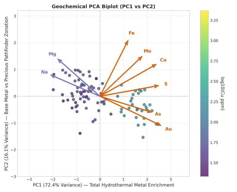
Exploration geologists frequently confuse dimensionality reduction with clustering. Principal component analysis geochemistry (PCA) is not a clustering method; rather, it is a linear transformation that projects multi-element data onto orthogonal principal components of maximum variance.
As outlined in the CRC LEME geochemical anomaly guide by McQueen, multivariate methods like PCA reduce multi-element correlations into primary components that explain major geochemical trends:
from sklearn.decomposition import PCA
import pandas as pd

def compute_geochemical_pca(clr_assay_df: pd.DataFrame, n_components: int = 3) -> tuple[pd.DataFrame, pd.DataFrame]:
    """Compute principal component loadings and transformed scores (educational example)."""
    pca = PCA(n_components=n_components)
    scores = pca.fit_transform(clr_assay_df)

    scores_df = pd.DataFrame(scores, columns=[f"PC{i+1}" for i in range(n_components)])
    loadings_df = pd.DataFrame(pca.components_.T, index=clr_assay_df.columns, columns=[f"PC{i+1}" for i in range(n_components)])

    return scores_df, loadings_df
In exploration workflows, geologists execute PCA prior to clustering to simplify multi-element matrices. However, PCA does not automatically separate analytical noise from geological signal; high variance may stem from background lithological shifts or analytical errors rather than mineralization.
Therefore, geologists must inspect explained variance ratios and element loadings before interpreting components. For example, three components explaining 80 percent of variance is a project-specific observation rather than a universal standard.
K-means, DBSCAN and PCA compared
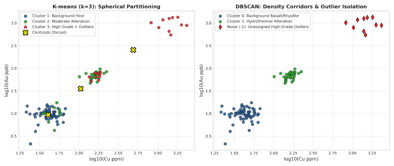
Selecting the appropriate mathematical method requires matching algorithmic properties to the structural geometry of the geochemical dataset. The comparative matrix below outlines key operational differences:
| Analytical Method | Algorithm Type | Requires Cluster Count k | Handles Density Outliers | Geometric Assumption | Primary Geological Failure Mode |
|---|---|---|---|---|---|
| K-Means | Centroid-based partitioning | Yes (declared by user) | Forces all outliers into nearest cluster | Spherical, equal-variance clusters | Merges narrow mineralized veins into broad host rock units |
| DBSCAN | Density-based partitioning | No (derived from density parameters) | Isolates sparse points as unassigned (-1) | Arbitrary, non-linear geometries | Misinterprets variable survey sample spacing as density shifts |
| PCA | Linear dimensionality reduction | No (orthogonal axis projection) | Outliers inflate component variance | Linear orthogonal axes | Fails to capture non-linear mineral associations across complex facies |
In practice, PCA serves as a complementary dimensionality-reduction tool before clustering rather than a direct alternative to K-means and DBSCAN. Combining PCA with density-based clustering often produces clearer alteration boundaries than clustering raw elements directly.
Worked example on an exploration traverse dataset
To demonstrate how these algorithms behave, consider a schematic exploration traverse across a volcanic-hosted massive sulfide prospect. Ten representative samples contain assayed concentrations of copper (Cu), gold (Au), arsenic (As), and molybdenum (Mo).
Exploration traverse assay dataset
The table below summarizes the multi-element assay values, algorithm assignments, and principal component scores for this schematic profile:
| Sample ID | Mapped Lithology | Cu (ppm) | Au (ppb) | As (ppm) | Mo (ppm) | K-Means (k = 3) | DBSCAN Label | PCA Score (PC1) |
|---|---|---|---|---|---|---|---|---|
| S-01 | Basalt Host | 45 | 8 | 4 | 1 | Cluster 1 | Cluster 0 | -1.84 |
| S-02 | Basalt Host | 52 | 12 | 6 | 2 | Cluster 1 | Cluster 0 | -1.62 |
| S-03 | Basalt Host | 48 | 10 | 5 | 1 | Cluster 1 | Cluster 0 | -1.75 |
| S-04 | Chlorite Alteration | 145 | 45 | 18 | 4 | Cluster 2 | Cluster 1 | 0.15 |
| S-05 | Chlorite Alteration | 180 | 60 | 22 | 5 | Cluster 2 | Cluster 1 | 0.48 |
| S-06 | Sericite Alteration | 120 | 85 | 48 | 12 | Cluster 2 | Cluster 1 | 0.82 |
| S-07 | Quartz Vein | 850 | 420 | 180 | 35 | Cluster 3 | Noise (-1) | 3.12 |
| S-08 | Massive Sulfide | 2400 | 1250 | 450 | 85 | Cluster 3 | Noise (-1) | 5.84 |
| S-09 | Rhyolite Tuff | 18 | 4 | 2 | 1 | Cluster 1 | Cluster 0 | -2.45 |
| S-10 | Rhyolite Tuff | 22 | 6 | 3 | 2 | Cluster 1 | Cluster 0 | -2.31 |
Comparing algorithm partitions and PCA scores
This schematic dataset illustrates key behavioral differences across algorithms under standardized parameters:
- Background grouping across distinct lithologies: Both barren basalt (S-01 to S-03) and barren rhyolite (S-09, S-10) group into Cluster 1 (K-means) and Cluster 0 (DBSCAN). Because this feature subset contains only base and precious metals without major rock-forming oxides (SiO₂, MgO), the algorithms group them by their shared lack of mineralization.
- Centroid distortion versus density isolation: K-means forces high-grade samples S-07 and S-08 into Cluster 3 alongside moderate assays. In contrast, DBSCAN labels them as unassigned density outliers (
-1) because their extreme concentrations place them outside dense background neighborhoods in 4D space. - Interpreting PCA component scores: In this example, PC1 accounts for 78 percent of total variance, with strong positive loadings across all elements (Cu: +0.52, Au: +0.55, As: +0.48, Mo: +0.44). Consequently, positive PC1 scores correlate with overall metal enrichment in this specific dataset, though component signs in PCA are mathematically arbitrary.
Geochemical anomaly detection: validating exploration clusters
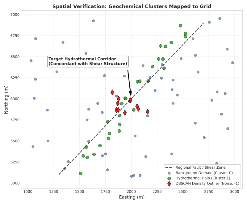
A mathematical clustering output is not self-validating. Exploration geologists must verify that identified clusters reflect physical geological reality rather than mathematical artifacts.
Validation protocols for exploration clustering
Geologists apply systematic validation workflows to assess cluster reliability:
- Map clusters in geographic space: Plot cluster assignments onto surface maps and cross-sections. While coherent spatial zones provide encouraging support, geologists must verify that spatial coherence does not simply mirror survey drill spacing or spatial autocorrelation.
- Compare against primary logging: Cross-reference cluster boundaries against mapped lithology and core photography. Clusters that cross-cut stratigraphic units should correspond to observable alteration, oxidation, or structural overprints.
- Test parameter stability: Re-run algorithms across varying parameter values (such as shifting k or adjusting ε) and measure partition stability using the Adjusted Rand Index. Consistent geological domains persist across parameter sweeps, whereas fragile artifacts disappear.
- Integrate with anomaly detection: Verify whether unassigned density outliers represent authentic mineralization by cross-referencing samples with formal geochemical anomaly detection models.
Additionally, exploration teams orchestrate these spatial checks within an autonomous geology AI agent to evaluate multivariate assay continuity across regional drill programs.
Chemical feature space versus spatial coordinates
A common dilemma in geochemical data clustering is whether to include spatial coordinates (X, Y, Z) alongside chemical assays. The table below outlines the analytical trade-offs:
| Clustering Space | Input Features | Primary Advantage | Analytical Risk |
|---|---|---|---|
| Pure Chemical Space | Multi-element clr assays only | Identifies identical rock units or alteration facies across dislocated fault blocks | May produce spatially scattered clusters that lack geographic continuity |
| Spatially Constrained Space | Assays plus scaled coordinates (X, Y, Z) | Enforces geographic contiguity, creating compact, mappable domains | Artificially merges chemically distinct rock units simply because they are adjacent |
In most early-stage exploration programs, clustering in pure chemical space first and using spatial coordinates strictly for independent validation yields the most defensible geological interpretations.
Geochemical data clustering in AI-assisted software
Modern exploration teams increasingly deploy automated machine learning pipelines within integrated software environments. Software suites designed for AI in mineral exploration streamline compositional transformations, algorithm selection, and 3D spatial mapping.
Specialized platforms like geology data analysis software integrate multi-element clustering with downhole drillhole databases. By connecting automated clustering directly to interactive voxel models, exploration geologists can visualize hydrothermal alteration envelopes in three dimensions while preserving full data provenance.
Furthermore, exploration geologists deploy geochemical clustering and anomaly tools to run unsupervised workflows like K-means, DBSCAN, and PCA directly on multi-element surveys while maintaining strict evidence traceability.
FAQs
What is clustering in geochemistry?
Clustering in geochemistry is an unsupervised machine learning process that groups rock or soil samples based on multi-element chemical similarities. It identifies natural geochemical domains, alteration halos, and lithological units without requiring prior manual labeling or subjective classification.
What is the difference between K-means and DBSCAN?
K-means partitions data into a user-specified number of spherical clusters and assigns every sample to a group. In contrast, DBSCAN determines cluster counts automatically based on sample density, accommodates irregular non-linear shapes, and explicitly isolates background outliers as noise.
Is PCA a clustering method?
No, principal component analysis is a linear dimensionality reduction method, not a clustering algorithm. Geologists use PCA before clustering to reduce dozens of correlated chemical elements into a few orthogonal components that capture the majority of geochemical variance.
How many clusters should I choose for geochemical data?
When using K-means, determine cluster count using statistical heuristics like the elbow method, silhouette scores, and gap statistics. Always validate selected cluster counts against mapped geological lithologies and known hydrothermal alteration facies in the exploration area.
Should I scale geochemical data before clustering?
Yes, scaling is essential because major oxides are measured in percent while trace pathfinders are measured in parts per million or billion. Standardizing transformed variables ensures that abundant rock-forming elements do not mathematically overwhelm critical trace indicators.
How do below-detection values affect clustering?
Below-detection values introduce zero-inflation and left-censored boundaries that distort log-ratio transformations and distance metrics. Consequently, exploration geologists apply disciplined imputation methods, such as multiplicative log-normal replacement or expectation-maximization algorithms, before computing compositional centered log-ratios across multi-element datasets.
How do I know if my clusters are real?
Validate geochemical clusters by plotting them on geological maps, cross-sections, and core logs. Authentic geochemical clusters correspond to coherent spatial domains, stratigraphic units, or alteration corridors, whereas artificial mathematical clusters appear scattered randomly across geographic space without geological support.
Try It With Geocluster
GeoCluster is a browser-based AI agent for geological investigation, available in open-source and enterprise editions. It provides automated geochemical clustering and anomaly detection tools, grouping multi-element assays into coherent 3D domains while keeping every cluster traceable to raw laboratory measurements.