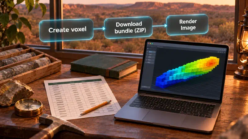
TL;DR: To import a voxel model into Blender, you use two tools: Geocluster builds the voxel grid from drilling tables, and Blender displays it. A drill hole is a borehole sampled for rock types and metal grades, while a voxel is a 3D grid cell storing one block value. Blender is a free 3D graphics program that converts the downloaded Geocluster bundle into a lit mesh render.
Why Visualise a Geological Voxel Model in Blender?
Geocluster lets geologists build, validate, and filter 3D grids directly in a web browser. When you need studio lighting, a custom camera angle, or a high-resolution figure, our geological modelling resource guides cover practical workflows for moving spatial data between tools.
In Blender you control the lighting, the background and the camera framing. None of that changes the values in the grid. Before building a 3D block grid, many teams start with a drill hole visualization workflow to inspect raw collar locations and downhole intervals.
The voxel built in this guide is a display construction for visual inspection only, not a physical measurement. It is neither a prospectivity model nor a mineral resource estimate, and it must not be used to estimate tonnes or rock volume.
What Is a Geocluster Voxel to Blender Conversion Workflow?
A voxel model divides a 3D block of ground into regular box-shaped cells along easting, northing, and depth axes. Each cell stores a numeric value and a validity flag indicating whether data exists at that grid index.
Geocluster has no GLB, glTF, or OBJ export and no direct Blender connector. To import a voxel model into Blender 3D creation suite, you use a local conversion workflow: a Python script in Blender reads the downloaded Geocluster ZIP bundle.
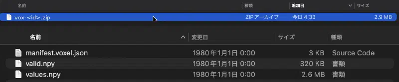
When you build a grid using the Existing grid mode in Geocluster, the downloaded ZIP archive holds three files: manifest.voxel.json, values.npy, and valid.npy. Because cell values are supplied directly rather than aggregated from raw sample points, the bundle does not include a counts.npy file.
The Blender importer script first checks the SHA-256 checksum of each .npy array against manifest.voxel.json. It then turns the NumPy grid into a mesh. To keep the mesh light, the script builds only the outer cube faces that touch an empty or filtered-out neighbour cell.
The voxel value used here, named Intersection footprint, combines three criteria from public drilling tables:
- High-grade gold cells where maximum detected
Auis at least0.1 ppm. - Target host-rock intervals where
Lithology1is one ofMB,M,MD,U,UTC,UTCB, orUPX. - Logged alteration share from non-blank
Alt1_Mineralrecords, combined as high-grade times lithology times(0.5 + 0.5 * alteration).
That 3D layer is folded over depth by taking its vertical maximum, smoothed horizontally with a 5-cell Gaussian filter (about 350 m), and cut to the strongest 12 percent of the horizontal window. Each kept column then restores vertical variation across all eight depth levels, producing relative screening values for visual inspection only.
Data Used in This Geocluster Voxel Guide
This walkthrough uses public open-file drilling tables from report A114051 (Central Laverton) in the Western Australian WAMEX database. We credit the Department of Energy, Mines, Industry Regulation and Safety, Government of Western Australia, as the source of this public dataset.
Three tab-separated WAMEX template files provide the inputs:
CL_WADL4_COLL2017A.txtfor drill collar coordinates and orientations.CL_WADL4_ASSAY2017A.txtfor downhole gold assay intervals (24 MB).CL_WADL4_GEOL2017A.txtfor downhole lithology and alteration logs.
In each file, lines starting with H hold header metadata, the line starting with H1000 holds the column names, and rows starting with D hold the data records. Collar coordinates use Map Grid of Australia Zone 51 in the EPSG:28351 MGA zone 51 coordinate reference system.
Intervals are placed at their midpoint along a straight line projected from the collar Dip and Azimuth_TRUE values (blank dip is treated as vertical; blank azimuth is treated as 0). Downhole survey tables are not used, and the vertical axis represents depth below the collar (0 to 80 m) rather than elevation above sea level.
Reading the lithology codes MB, M, MD, U, UTC, UTCB, and UPX as mafic or ultramafic rocks is our own assumption and is not confirmed with a company legend. Below-detection entries, blanks, and negative assay codes are treated as not detected rather than replaced with zero.
Our test run on the 14 km by 14 km study window (E 437000 to 451000, N 6805000 to 6819000) builds a 200 x 200 x 8 grid of 70 m x 70 m x 10 m cells with these counts and value ranges:
| Test Run Metric | Test Run Value |
|---|---|
| Collars inside study window | 1,098 (of 1,805 collar rows) |
| Intervals inside grid | 32,206 of 71,238 assay midpoints; 9,540 of 25,842 geology midpoints |
Grid dimensions (x, y, z) | 200 x 200 x 8 (320,000 total cells) |
| Cell dimensions | 70 m x 70 m x 10 m |
| Depth range below collar | 0 to 80 m (z = 0 is 70 to 80 m; z = 7 is 0 to 10 m) |
High-grade cells (Au >= 0.1 ppm) | 245 (from 3,757 cells with detected Au and 5,999 cells with assay data) |
Product layer (Au x lithology x alteration) | 15,847 cells above zero (23,658 non-empty cells, maximum 0.358) |
Final CSV (x,y,z,intersection_footprint) | 38,400 rows (4,800 columns x 8 depth levels) |
intersection_footprint value range | 0.0012357 to 0.0691373 |
Cells at or above 0.01 | 11,495 |
How to Import Voxel Model Into Blender From Geocluster
Step 1: Build the Voxel CSV With Four AI Agent Prompts
You can run the four prompts in sequence inside your coding agent to build the x,y,z,intersection_footprint CSV from the three WAMEX text files. After the agent finishes, compare the cell count and value range from the agent with the test run numbers in the table above and the step notes below.
The CL_WADL4_ASSAY2017A.txt file is 24 MB. If the 24 MB assay file is refused when you upload it to the agent, trim the assay file before uploading to keep only the H header lines, the H1000 column row, and seven columns: Hole_id, Depth From, Depth To, Au_FA25_ppm, Au_Au_AA26_ppm, Au_FAA505_ppm, and Au_Au_ICP22_ppm, and state that trim in your report.
Paste these four prompts in order, one at a time. Each box is one prompt.
Prompt 1: Check the Files
Read CL_WADL4_COLL2017A.txt, CL_WADL4_ASSAY2017A.txt and CL_WADL4_GEOL2017A.txt. They are tab-separated WAMEX templates: lines starting with H are header metadata, the line starting with H1000 holds the column names, and rows starting with D are data. Report the number of data rows in each file, the column names, and how many holes in the assay and geology files have no collar. Do not change any file.Prompt 2: Place Each Interval in a 3D Cell
Use MGA Easting and MGA Northing from the collar file in EPSG:28351. Place each assay and geology interval at its midpoint along a straight hole from the collar Dip and Azimuth_TRUE (blank dip means vertical, blank azimuth means 0). Do not use downhole surveys. Use a window of E 437000 to 451000 and N 6805000 to 6819000, cells 70 m by 70 m horizontally and 10 m vertically, and depth 0 to 80 m below the collar, giving a 200 by 200 by 8 grid. Report how many collars fall in the window and how many intervals fall in the grid. Do not invent missing collars.Prompt 3: Build the Screening Values
For Au use the first non-blank value of Au_FA25_ppm, Au_Au_AA26_ppm, Au_FAA505_ppm, Au_Au_ICP22_ppm. Treat blanks, below-detection values and negative codes as not detected and leave them out; do not replace them with zero. Mark a cell high-grade (1) when its maximum detected Au is at least 0.1 ppm, and 0 when it has detected Au below that; cells with no detected Au are not observed. From the geology file take the share of intervals per cell whose Lithology1 is one of MB, M, MD, U, UTC, UTCB, UPX (read as mafic or ultramafic, an assumption) and the share with a non-blank Alt1_Mineral. Smooth the high-grade indicator, the lithology share and the alteration share each in x and y with a Gaussian of 3 cells, weighting by observed cells only (assay-observed cells for the high-grade indicator, cells with geology intervals for the two shares) so empty neighbours do not count as zero. Then multiply smoothed high-grade by smoothed lithology share by (0.5 + 0.5 times smoothed alteration share) at each depth level, and leave a cell empty when its smoothed assay weight is below 0.05 of full weight. State every choice in the report.Prompt 4: Fold the Layer Into a Footprint and Write the CSV
Use cell_product_corrected.csv as the layer (not the earlier cell_product.csv). Treat cells with no product value as 0. Take the maximum over depth of the layer for each column, smooth it with a plain Gaussian of 5 cells in x and y (kernel truncated at 15 cells, empty space outside the grid counts as 0, do not renormalise by the amount of data), and keep the strongest 12 percent of the 200 by 200 window (4,800 columns, ties broken by lower x, then lower y). For each kept column, give all 8 levels the value smoothed maximum times (0.5 + 0.5 times the layer at that level divided by its maximum over depth); where that maximum is 0, use a ratio of 0 for all levels. Write a CSV with the columns x, y, z, intersection_footprint, using 0-based cell indices, one row per non-zero cell, with z index 0 as the deepest level (70 to 80 m) and 7 the surface. Save the CSV exactly the way you saved cell_product_corrected.csv. Name it intersection_footprint.indexed.csv and put it in the same results folder. Do not type the rows into a text-write tool. If saving needs my approval for the exact path, ask me for it and wait. After saving, read the file back and report its row count, its value range and the number of distinct (x, y) columns. If you really cannot save it that way, say which step failed and stop. Also save a short Markdown report with the cell counts, the value range and every assumption.What the Agent Reported in Prompts 1 to 3
In our run on the three WAMEX tables, Prompt 1 reported 1,805 collar rows, 71,238 assay rows, 25,842 geology rows, and 0 holes without a collar. The collar ID column is Hole_ID, while the assay and geology ID column is Hole_id; the agent matched them with an exact, case-sensitive check. Prompt 2 found 1,098 collars inside the study window, placed 32,206 of 71,238 assay midpoints and 9,540 of 25,842 geology midpoints inside the grid, and dropped no intervals for a missing collar.
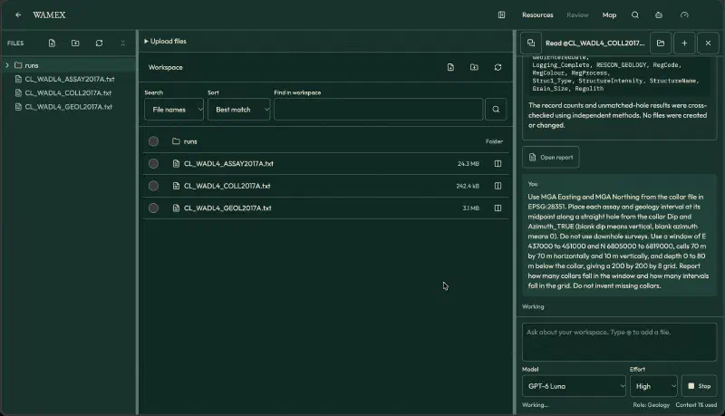
Prompt 3 was reworded during testing into the final box above. Our first wording only smoothed the lithology and alteration shares, so the high-grade indicator stayed unsmoothed and the layer came out much smaller than intended. The agent’s first answer also used measured downhole depth instead of vertical depth below the collar, and it corrected this when checked. Always check how your agent turns interval depth into vertical depth below the collar.
In the corrected Prompt 3 run, 5,999 cells held assay data, 3,757 had detected Au, and 245 were high-grade. Cells without detected Au are left empty, not set to zero. Of the 9,540 in-grid geology intervals, 964 had a target lithology code and 697 had a non-blank Alt1_Mineral. The saved product table (cell_product_corrected.csv) had 23,658 non-empty cells, 15,847 of them above zero, with a maximum of 0.358.
What Happened With Prompt 4
We ran Prompts 1 to 3 with GPT-6 Luna (effort High). In Prompt 4, the agent computed the footprint table but could not write the 38,400-row file, first with a short save instruction and again after we changed the wording. The save worked once we switched the model to Gemini 3.8 Flash and told it to save intersection_footprint.indexed.csv the same way it saved cell_product_corrected.csv, without typing rows into a text-write tool. We did not test the new wording on its own, so we cannot say whether the model or the wording made the difference. If your agent cannot save a large table, try both. The saved CSV read back with 38,400 rows, 0 duplicate cells, 4,800 distinct (x, y) columns, z from 0 to 7, values from 0.0012357 to 0.0691373, and 11,495 cells at or above 0.01.
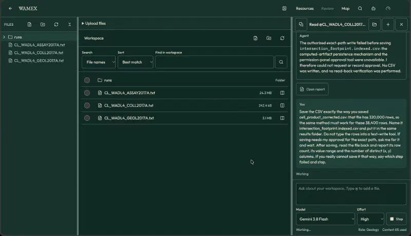
The table in the data section comes from this run. We recomputed the same CSV independently and compared it with a footprint from our own script: 96% of the 4,800 kept columns coincide, and the blobs sit in the same places. Your agent’s counts should land close to the table. A few percent of difference is fine if the footprint sits in the same places.
Step 2: Create the Voxel Grid in Geocluster and Download the ZIP Bundle
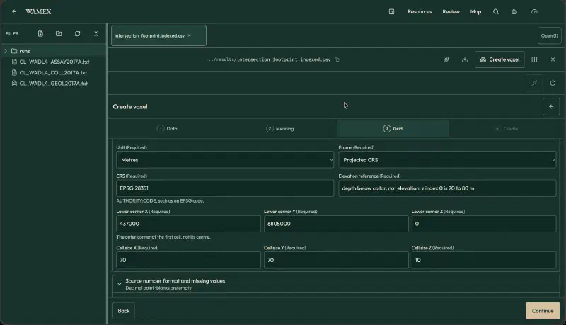
Open the Create voxel wizard in Geocluster, which steps through Data, Meaning, Grid, and Create. Upload your CSV in the Data step and select Existing grid in the Meaning step so Geocluster loads values already assigned to grid cells.
Configure the Meaning and Grid steps with these exact settings:
| Wizard Control | Setting | Notes |
|---|---|---|
| Meaning option | Existing grid | Loads pre-assigned cell indices and values |
| Index columns | x, y, z | Mapped to grid cell indices |
| Value field | intersection_footprint | Displayed in the voxel as Intersection footprint |
| First index | 0 | Matches 0-based indices from the CSV |
| Cell occupancy | Allow empty cells | Chosen instead of Every cell has a value |
| Grid shape | 200 x 200 x 8 | 200 easting by 200 northing by 8 depth cells |
| Cell size | 70 x 70 x 10 m | Covers 14,000 m by 14,000 m by 80 m |
| Horizontal CRS | EPSG:28351 | MGA Zone 51 horizontal coordinates |
| Lower corner | 437000, 6805000, 0 | Outer corner of the first cell (0, 0, 0) |
| Elevation reference | depth below collar, not elevation; z index 0 is 70 to 80 m | Free text note; vertical datums are not converted |
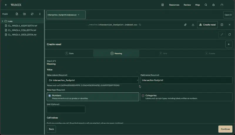
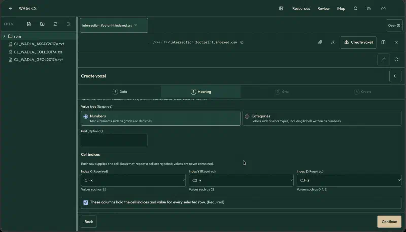
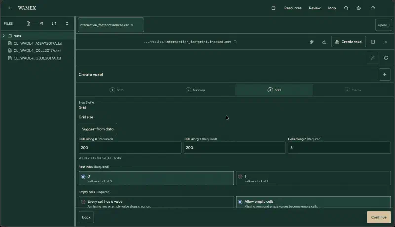
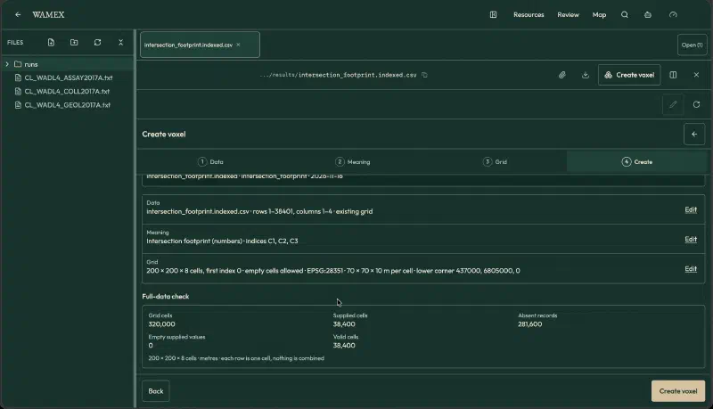
In the Create step, run Full-data check to verify cell indexing before building the 3D view. On this CSV, Full-data check shows 320,000 grid cells, 38,400 supplied cells, 281,600 absent records, 0 empty supplied values, and 38,400 valid cells.
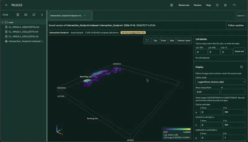
Click Open in 3D to inspect the voxel inside Geocluster. Set the colour scale to Logarithmic (shown cells), set vertical exaggeration to 10x, and enter 0.01 in the Show values from filter field. The viewer shows 11,495 of 38,400 occupied cells shown, with a data range of 0.00123570049 to 0.06913732692 and a legend from 0.01 to 0.06914.
If the panel shows Keep this version, click it to save the grid state, then click Download bundle (ZIP). The downloaded ZIP file contains manifest.voxel.json, values.npy, and valid.npy. Do not unzip the download (some browsers unzip files automatically, so turn that setting off), because the Blender script reads the .zip file itself and stops with the ZIP_PATH message if you point it at a folder.
Step 3: Import the Voxel ZIP Bundle in the Blender Scripting Workspace
Open Blender, switch to the Scripting workspace at the top of the window, and paste import_voxel_blender_indexed.py into a new text block in the Text Editor:
"""Import a Geocluster voxel ZIP (values.npy + valid.npy) into Blender as colored cubes.

Only faces next to an empty cell are built, so large grids stay light.
Set ZIP_PATH, then Run Script in Blender's Scripting workspace.
"""
import hashlib
import io
import json
import zipfile
from pathlib import Path

import bpy
import numpy as np

ZIP_PATH = "/full/path/to/your-voxel.zip"
OBJECT_NAME = "Geocluster_Footprint_Voxels"
VERTICAL_EXAGGERATION = 10.0   # the layer is 80 m thick and 14 km wide
MIN_VALUE = 0.01               # raise to remove weak cells; lower to show more of the footprint
LOG_SCALE = True
PALETTE = ((0.10, 0.20, 0.45, 1), (0.10, 0.45, 0.60, 1), (0.15, 0.65, 0.55, 1),
           (0.60, 0.80, 0.30, 1), (1.00, 0.85, 0.10, 1))


def read(archive, manifest, role):
    rec = next(a for a in manifest["arrays"] if a["role"] == role)
    data = archive.read(role + ".npy")
    if hashlib.sha256(data).hexdigest() != rec["sha256"]:
        raise ValueError(f"Checksum mismatch for {role}.npy")
    return np.load(io.BytesIO(data), allow_pickle=False)


if not Path(ZIP_PATH).is_file():
    raise FileNotFoundError(f"Set ZIP_PATH to your voxel ZIP: {ZIP_PATH}")
with zipfile.ZipFile(ZIP_PATH) as z:
    manifest = json.loads(z.read("manifest.voxel.json"))
    values = read(z, manifest, "values")
    valid = read(z, manifest, "valid").astype(bool)

grid = manifest["grid"]
shape, spacing, origin = tuple(grid["shape"]), np.array(grid["spacing"], float), np.array(grid["origin"], float)
if values.shape != shape or valid.shape != shape:
    raise ValueError("Array shape does not match the manifest")
show = valid & (values >= MIN_VALUE)
if not show.any():
    raise ValueError("No cells to show; lower MIN_VALUE")

vals = values[show]
lo, hi = float(vals.min()), float(vals.max())
t = (np.log(vals) - np.log(lo)) / (np.log(hi) - np.log(lo)) if LOG_SCALE and lo > 0 and hi > lo else (vals - lo) / max(hi - lo, 1e-12)
band = np.minimum((t * len(PALETTE)).astype(int), len(PALETTE) - 1)
bands = np.zeros(shape, int)
bands[show] = band

# Scene scale: centre on the grid, stretch z.
scale = spacing * np.array([1, 1, VERTICAL_EXAGGERATION])
center = (origin + np.array(shape) * spacing / 2) * np.array([1, 1, VERTICAL_EXAGGERATION])

# Face = (neighbour offset, 4 corners of the unit cube face, counter-clockwise from outside)
FACES = [((-1, 0, 0), [(0, 0, 0), (0, 0, 1), (0, 1, 1), (0, 1, 0)]),
         ((1, 0, 0), [(1, 0, 0), (1, 1, 0), (1, 1, 1), (1, 0, 1)]),
         ((0, -1, 0), [(0, 0, 0), (1, 0, 0), (1, 0, 1), (0, 0, 1)]),
         ((0, 1, 0), [(0, 1, 0), (0, 1, 1), (1, 1, 1), (1, 1, 0)]),
         ((0, 0, -1), [(0, 0, 0), (0, 1, 0), (1, 1, 0), (1, 0, 0)]),
         ((0, 0, 1), [(0, 0, 1), (1, 0, 1), (1, 1, 1), (0, 1, 1)])]
pad = np.pad(show, 1)
idx = np.argwhere(show)
verts, mats = [], []
for (dx, dy, dz), corners in FACES:
    nb = pad[idx[:, 0] + 1 + dx, idx[:, 1] + 1 + dy, idx[:, 2] + 1 + dz]
    cells = idx[~nb]                      # cells whose neighbour is empty or outside
    base = origin + cells * spacing
    for c in corners:
        verts.append((base + np.array(c) * spacing) * np.array([1, 1, VERTICAL_EXAGGERATION]) - center)
    mats.append(bands[tuple(cells.T)])
n_per = [len(m) for m in mats]
# Interleave per face group: vertices of each corner list are stored corner-major, so rebuild.
all_verts, loops, face_mat, offset = [], [], [], 0
for g, ((_, corners), n) in enumerate(zip(FACES, n_per)):
    block = np.stack(verts[g * 4:(g + 1) * 4], axis=1).reshape(-1, 3)   # (n*4, 3), 4 per face
    all_verts.append(block)
    loops.append(np.arange(n * 4).reshape(n, 4) + offset)
    face_mat.append(mats[g])
    offset += n * 4
# 1 Blender unit = 100 m, so the 14 km grid stays inside the viewport clip distance.
all_verts = (np.concatenate(all_verts) * 0.01).astype(np.float32)
loops = np.concatenate(loops).astype(np.int32)
face_mat = np.concatenate(face_mat).astype(np.int32)
nf = len(loops)

for old in list(bpy.data.objects):
    if old.name == OBJECT_NAME or old.name.startswith(OBJECT_NAME + "."):
        bpy.data.objects.remove(old, do_unlink=True)

mesh = bpy.data.meshes.new(OBJECT_NAME + "_Mesh")
mesh.vertices.add(len(all_verts))
mesh.vertices.foreach_set("co", all_verts.ravel())
mesh.loops.add(nf * 4)
mesh.loops.foreach_set("vertex_index", loops.ravel())
mesh.polygons.add(nf)
mesh.polygons.foreach_set("loop_start", np.arange(nf, dtype=np.int32) * 4)
mesh.polygons.foreach_set("loop_total", np.full(nf, 4, np.int32))
mesh.update()
mesh.validate()

for i, color in enumerate(PALETTE):
    m = bpy.data.materials.new(f"Footprint band {i + 1}")
    m.use_nodes = True
    m.diffuse_color = color
    p = m.node_tree.nodes.get("Principled BSDF")
    if p:
        p.inputs["Base Color"].default_value = color
    mesh.materials.append(m)
mesh.polygons.foreach_set("material_index", face_mat)
mesh.update()

obj = bpy.data.objects.new(OBJECT_NAME, mesh)
bpy.context.collection.objects.link(obj)
obj["field"] = manifest["field"]["name"]
obj["value_min"], obj["value_max"] = lo, hi
obj["shown_cells"] = int(show.sum())
obj["horizontal_crs"] = grid["horizontalReference"]["definition"]
obj["vertical_reference"] = grid["verticalReference"]
obj["vertical_exaggeration"] = VERTICAL_EXAGGERATION

bpy.ops.object.select_all(action="DESELECT")
obj.select_set(True)
bpy.context.view_layer.objects.active = obj
for area in bpy.context.screen.areas:
    if area.type == "VIEW_3D":
        with bpy.context.temp_override(area=area, region=next(r for r in area.regions if r.type == "WINDOW")):
            bpy.ops.view3d.view_selected()
print(f"{int(show.sum())} cells, {nf} faces, value {lo:.4g} to {hi:.4g}")
At the top of the importer script, set ZIP_PATH to /full/path/to/your-voxel.zip and leave MIN_VALUE at its default of 0.01. Click Run Script in the Text Editor header to execute the conversion workflow.
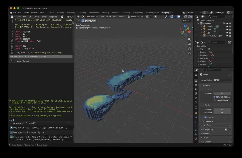
Before building geometry, the script validates the bundle and raises specific messages if checks fail:
| Error Message | Cause and Fix |
|---|---|
Set ZIP_PATH to your voxel ZIP: ... | The path in ZIP_PATH does not exist; update /full/path/to/your-voxel.zip to match your downloaded file location. |
Checksum mismatch for <role>.npy | The SHA-256 hash of values.npy or valid.npy does not match manifest.voxel.json; download a fresh ZIP bundle. |
Array shape does not match the manifest | The dimensions inside the .npy array disagree with the grid shape in manifest.voxel.json. |
No cells to show; lower MIN_VALUE | No valid cells have values at or above MIN_VALUE; lower the threshold and run the script again. |
When validation passes at MIN_VALUE = 0.01, the script creates a mesh object named Geocluster_Footprint_Voxels containing 11,495 cells, matching the filtered count in the Geocluster viewer, and prints 11495 cells (with the face count and value range) to the Blender system console, not the interactive Python console. It converts coordinates at a scale of 1 Blender unit = 100 m with a vertical exaggeration of 10, and builds only cube faces next to an empty cell.
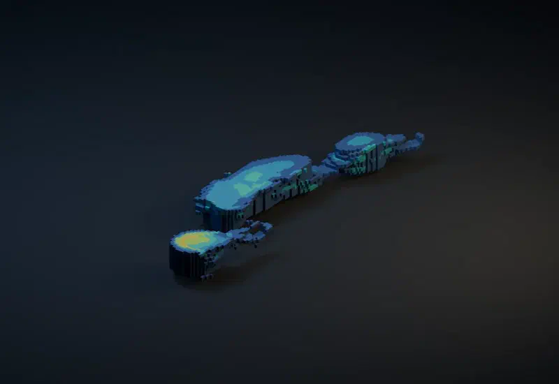
The importer also creates five materials, one for each colour band. Switch the viewport to Material Preview to see them. Those five colour bands show relative position within the visible value range and are not a calibrated gold grade legend.
Step 4: Inspect Custom Properties and Render the Scene
Select Geocluster_Footprint_Voxels in the Outliner, move your cursor into the 3D Viewport, and press Numpad . (View > Frame Selected) to frame the mesh. Switch the viewport shading mode to Material Preview or Rendered to see the five relative colour bands across the 11,495 cells.
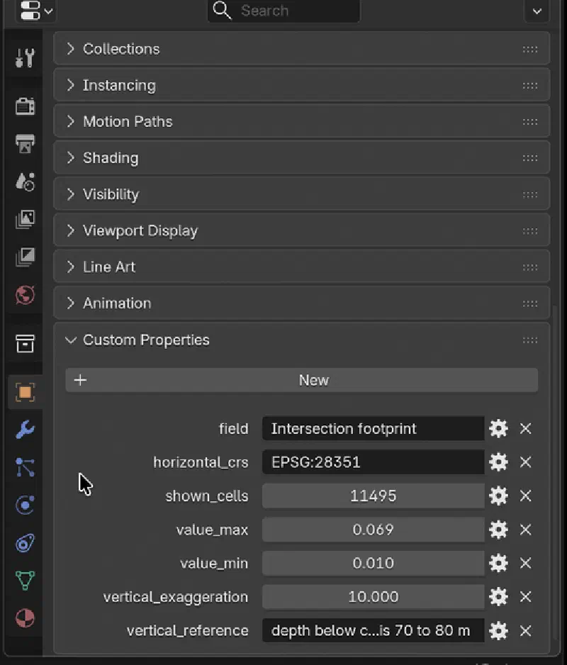
To find the metadata attached by the importer, click Geocluster_Footprint_Voxels in the Outliner, open the Object tab (orange square icon) in the Properties panel, and scroll down to Custom Properties. Blender shows decimal values rounded (0.010 and 0.069) and cuts off long text, so widen the Properties panel (hover over it and press Ctrl+Space) before taking a screenshot:
| Custom Property Name | Value on Imported Voxel |
|---|---|
field | Intersection footprint |
value_min | 0.0100002 (smallest value among the 11,495 shown cells at or above MIN_VALUE of 0.01; shown as 0.010 in the panel) |
value_max | 0.0691373 (largest shown value; shown as 0.069 in the panel) |
shown_cells | 11495 |
horizontal_crs | EPSG:28351 |
vertical_reference | depth below collar, not elevation; z index 0 is 70 to 80 m |
vertical_exaggeration | 10.0 |
Before running the render setup script, delete the default Cube and Light in the 3D Viewport (click each object, press X, and choose Delete; the default Camera can stay because the script sets its own active camera). Next, paste render_voxel_scene.py into a new text block, check that VOXEL_NAME at the top matches "Geocluster_Footprint_Voxels", and click Run Script:
"""Set a camera, dark background, floor and lights for the imported Geocluster voxel."""
import bpy
from mathutils import Vector

VOXEL_NAME = "Geocluster_Footprint_Voxels"
OUTPUT = "//geocluster-voxel-render.png"

voxel = bpy.data.objects.get(VOXEL_NAME)
if voxel is None:
    raise RuntimeError(f"Can't find {VOXEL_NAME}. Run the indexed voxel importer first.")

# Idempotently replace only this script's camera, lights and ground.
for name in ("GeoVoxel_Camera", "GeoVoxel_Key", "GeoVoxel_Fill", "GeoVoxel_Ground"):
    obj = bpy.data.objects.get(name)
    if obj:
        bpy.data.objects.remove(obj, do_unlink=True)

corners = [voxel.matrix_world @ Vector(corner) for corner in voxel.bound_box]
lo = Vector(tuple(min(v[i] for v in corners) for i in range(3)))
hi = Vector(tuple(max(v[i] for v in corners) for i in range(3)))
center = (lo + hi) * 0.5
span = max(hi.x - lo.x, hi.y - lo.y)
if span <= 0:
    raise RuntimeError("Voxel has no horizontal extent")

# Dark ground plane just below the block, for a soft contact shadow.
bpy.ops.mesh.primitive_plane_add(size=span * 5, location=(center.x, center.y, lo.z - span * 0.025))
ground = bpy.context.object
ground.name = "GeoVoxel_Ground"
mat = bpy.data.materials.new("GeoVoxel_DarkGround")
mat.diffuse_color = (0.012, 0.020, 0.035, 1)
mat.use_nodes = True
mat.node_tree.nodes["Principled BSDF"].inputs["Base Color"].default_value = mat.diffuse_color
mat.node_tree.nodes["Principled BSDF"].inputs["Roughness"].default_value = 0.92
ground.data.materials.append(mat)

# Camera above and to the south-east, looking at the volume from an oblique angle.
bpy.ops.object.camera_add(location=center + Vector((span * 0.95, -span * 1.25, span * 0.90)))
camera = bpy.context.object
camera.name = "GeoVoxel_Camera"
camera.rotation_euler = (center - camera.location).to_track_quat("-Z", "Y").to_euler()
camera.data.type = "ORTHO"
camera.data.ortho_scale = span * 1.60
bpy.context.scene.camera = camera

# Light power scales with span squared: the lights sit about one span away,
# and light falls off with the square of distance.
def area_light(name, location, energy, color, size):
    data = bpy.data.lights.new(name, "AREA")
    data.energy, data.color, data.shape, data.size = energy, color, "DISK", size
    obj = bpy.data.objects.new(name, data)
    bpy.context.collection.objects.link(obj)
    obj.location = location
    obj.rotation_euler = (center - obj.location).to_track_quat("-Z", "Y").to_euler()
    return obj

area_light("GeoVoxel_Key", center + Vector((-span * 0.55, -span * 0.40, span * 1.25)), 14 * span ** 2, (0.60, 0.78, 1.0), span * 0.9)
area_light("GeoVoxel_Fill", center + Vector((span * 0.70, span * 0.30, span * 0.65)), 7 * span ** 2, (1.0, 0.68, 0.32), span * 0.7)

world = bpy.data.worlds.new("GeoVoxel_DarkWorld") if bpy.data.worlds.get("GeoVoxel_DarkWorld") is None else bpy.data.worlds["GeoVoxel_DarkWorld"]
bpy.context.scene.world = world
world.use_nodes = True
world.node_tree.nodes["Background"].inputs["Color"].default_value = (0.004, 0.008, 0.018, 1)
world.node_tree.nodes["Background"].inputs["Strength"].default_value = 0.25

# Keep the vivid five-band palette legible under the render lighting.
palette = ((0.035, 0.10, 0.35, 1), (0.02, 0.34, 0.56, 1), (0.02, 0.62, 0.48, 1),
           (0.48, 0.78, 0.10, 1), (1.0, 0.72, 0.02, 1))
for index, color in enumerate(palette, 1):
    material = bpy.data.materials.get(f"Footprint band {index}")
    if material:
        material.diffuse_color = color
        material.use_nodes = True
        shader = material.node_tree.nodes.get("Principled BSDF")
        if shader:
            shader.inputs["Base Color"].default_value = color
            shader.inputs["Roughness"].default_value = 0.72

scene = bpy.context.scene
scene.render.engine = "BLENDER_EEVEE"
scene.render.resolution_x, scene.render.resolution_y = 1600, 1100
scene.render.resolution_percentage = 100
scene.render.image_settings.file_format = "PNG"
scene.render.film_transparent = False
scene.render.filepath = OUTPUT
scene.view_settings.view_transform = "AgX"
scene.camera.data.lens = 50

print(f"Voxel scene ready. Render with F12; output: {OUTPUT}")
The script creates four scene objects (GeoVoxel_Camera, GeoVoxel_Key, GeoVoxel_Fill and GeoVoxel_Ground) and a dark world background. The model is about 105 Blender units wide, and light falls off with the square of distance, so a fixed light power gave a black image. The script sets the power of the two area lights to 14 and 7 times the span squared.
The render script sets the output resolution to 1600 x 1100 PNG and assigns the render engine to BLENDER_EEVEE because Blender 5.3 does not accept the BLENDER_EEVEE_NEXT engine name. In the top menu bar, click Render > Render Image (or press F12) to render the final frame, then choose Image > Save As in the render window to save the PNG, and File > Save to save the .blend file. The image is not saved automatically.
Limits of This Geocluster Voxel to Blender Workflow
- The voxel and its Blender render are for visual inspection only and must not be used as a mineral resource estimate or prospectivity model.
- The Geocluster grid and the Blender mesh are display constructions, not physical measurements, resource estimates, or prospectivity models. They must not be used to estimate tonnes or rock volume.
- Geocluster has no native GLB, glTF, or OBJ export and no Blender connector, so bringing a grid into Blender requires running the Python conversion workflow on the downloaded ZIP.
- The vertical grid axis is depth below collar (
0to80 m), not true elevation, so cells at the samezindex follow surface topography variations between collars. - Drill hole sample midpoints are projected along straight lines from collar dip and azimuth without downhole survey data.
- Treating the WAMEX lithology codes
MB,M,MD,U,UTC,UTCB, andUPXas mafic or ultramafic rocks is our reading and has not been verified against a company legend. - The
0.1 ppmgold threshold, the 3-cell and 5-cell Gaussian smoothing (~350 m), and the 12 percent area cutoff are screening parameters chosen to highlight multi-hole clusters. - The five material colours represent relative logarithmic bands across the
11,495shown cells (atMIN_VALUE = 0.01) rather than calibrated assay grades. - The scene setup script specifies
BLENDER_EEVEEfor compatibility with Blender 5.3, which rejectsBLENDER_EEVEE_NEXT.
FAQs
Does Geocluster Export GLB, glTF, or OBJ Files for Blender?
No, Geocluster does not export GLB, glTF, or OBJ meshes and has no direct Blender connector. Instead, you download the Geocluster voxel bundle as a ZIP file containing NumPy arrays and a JSON manifest. A Python script inside Blender reads those arrays and builds the 3D voxel mesh directly.
Why Does the Voxel ZIP Bundle Have No counts.npy File?
The ZIP bundle omits counts.npy because the voxel was created using the Existing grid option rather than point aggregation. Every supplied cell already carries a single pre-calculated value from the CSV file. Consequently, the downloaded archive only needs manifest.voxel.json, values.npy, and valid.npy to store the grid values and validity mask.
Is This Voxel a Resource Estimate?
No, this voxel is a display construction for visual inspection, not a measurement, resource estimate, or prospectivity model. You must not use the Geocluster grid or the Blender render to estimate tonnes or rock volume. The intersection footprint values are dimensionless numbers built from smoothed gold thresholds, assumed lithology groupings, and logged alteration shares.
Why Does the Blender Render Script Use BLENDER_EEVEE Instead of BLENDER_EEVEE_NEXT?
The render script sets scene.render.engine to BLENDER_EEVEE because Blender 5.3 does not accept the engine name BLENDER_EEVEE_NEXT. This scene setup was tested in Blender 5.3 using render_voxel_scene.py. Do not copy engine names from older tutorials.
Why Does the Importer Only Build Outer Cube Faces Next to Empty Cells?
The importer skips interior faces between touching cells to reduce polygon count and prevent rendering artefacts on internal boundaries. At a cutoff of 0.01, the filtered grid still contains 11,495 active cells. Generating only exposed boundary faces keeps the Blender viewport responsive while preserving the exact outer shape and colour bands.
What Should I Do if the AI Agent Upload Rejects the Assay File?
If the 24 MB CL_WADL4_ASSAY2017A.txt assay file is refused when you upload it to the agent, trim it before uploading. Keep the H header lines, the H1000 column header row, and only seven columns: Hole_id, Depth From, Depth To, Au_FA25_ppm, Au_Au_AA26_ppm, Au_FAA505_ppm, and Au_Au_ICP22_ppm. State that trim in your report.
Why Is My Blender Render Black?
Your Blender render is black because the lights are too weak for a model this wide. At about 105 Blender units across, light falls off with the square of distance. Run render_voxel_scene.py, which scales light power with the model width (14 and 7 times the span squared), or raise the Power of the two lights.
Import Voxel Model Into Blender With Geocluster
Validating your 3D grid in Geocluster first ensures cell counts, value ranges, and spatial metadata are checked before you spend time lighting a scene in Blender. Once you download the verified ZIP bundle, the Python conversion workflow builds the filtered mesh, preserves manifest metadata as custom properties, and sets up a repeatable studio render.
To test your own drilling grids and download verified voxel bundles, explore the Geocluster platform.