TL;DR: Want to interpolate geological surfaces between drillholes without writing code? A geological surface is the boundary between two rock layers, such as the top of hard basement rock under softer sediment. Drillholes tell you its depth only where they pass through it, so you estimate the depth everywhere else. In the Geocluster workspace, four prompts to the built-in AI agent pick that boundary in 47 public South Australian holes, estimate it three ways, test each way by hiding one hole at a time, and save the result as a map layer. The methods agree near the holes and disagree by up to 50 m away from them, so the map also shows where to trust it.
What Does It Mean to Interpolate Geological Surfaces?
A contact is the boundary between two rock units. Each drillhole gives its elevation at one point. To interpolate geological surfaces, you estimate that elevation on a grid between the holes, so the boundary becomes a continuous surface you can map, contour and use in a model.
You may also see this task written as interpolate between boreholes, interpolate geological contacts, or stratigraphic surface interpolation.
The key point is that you interpolate the geometry of a boundary, not the rock types. Averaging “sandstone” and “granite” between holes means nothing. In contrast, the elevation of the contact between them is a number that changes smoothly enough to estimate. We use elevation (RL, reduced level) rather than depth below the collar, because the collars sit at different heights.
Three common methods do the estimating:
- IDW (inverse distance weighting): each grid cell takes a weighted average of the holes, with nearer holes weighted more.
- RBF (radial basis function): a smooth mathematical surface, here a thin plate spline, bends to pass exactly through every hole.
- Kriging: a statistical method that first measures how quickly the surface changes with distance, then uses that to weight the holes and estimate its own error.
Part 1 of this series showed measured drill data with nothing interpolated. The previous parts matched and drew contacts by hand. This part is where the process becomes computational.
Drillhole Data Used in This Guide
We continue with the SARIG Data Package, the South Australian government’s public export of drilling records, and the Carrapateena project area from the previous guides. This time we use every hole in the area that has a stratigraphic log: 49 holes over about 2.2 by 1.8 km.
Download and Filter the SARIG Files
We cut the SARIG exports down to these holes and kept every column unchanged. To follow along, download the three full exports:
- sarig_dh_details_exp.csv (140 MB): position, elevation and depth of each hole
- sarig_dh_litho_exp.csv (402 MB): the rock intervals
- sarig_dh_strat_exp.csv (58 MB): the named unit intervals
In the details export, keep the holes with ZONE_GDA2020 53, EASTING_GDA2020 from 735,000 to 741,000, NORTHING_GDA2020 from 6,543,000 to 6,546,000 and STRAT_LOG equal to Y. That gives 49 holes. Then keep the rows of those DRILLHOLE_NO values in the other two exports, and save the three files as sarig_area_details.csv, sarig_area_litho.csv and sarig_area_strat.csv. These exports are large, so use a script or a tool built for large CSV files.
Source: The Department for Energy and Mining, the Government of South Australia, The SARIG Data Package, Sourced on 9 November 2026, https://dem-sdp.s3-ap-southeast-2.amazonaws.com/index.html.
Licensed under CC BY 4.0. We filtered the exports to 49 holes and derived the figures and map layers in this guide from them. The Government of South Australia does not endorse this guide.
Three things about this data shape the steps below:
- One surface. We map contact C4, the base of the sandstone and conglomerate cover where it rests on granite. It has the most relief of the contacts in the previous guides.
- A gap in the holes. Four holes sit about 840 m north-east of the main cluster, with no holes in between.
- Two ways of logging one contact. In some holes, the stratigraphic log puts the top of the granite at the top of the last conglomerate, not at its base, so the contact needs one consistent rule first.
How Do I Interpolate Geological Surfaces in Geocluster?
To interpolate geological surfaces between drillholes, send four prompts one at a time in the same conversation, and wait until each one finishes. The agent writes and runs the interpolation code in your workspace, and the result opens as a layer in the Geocluster map.
Step 1: Pick the Contact in Every Hole
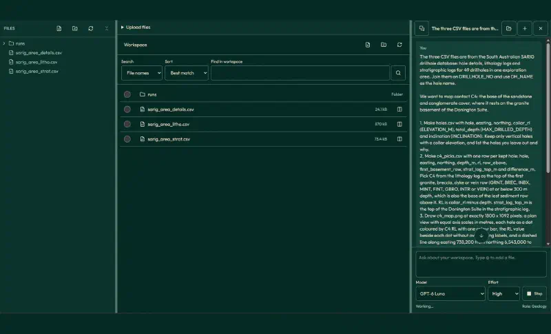
First, upload the three area files to a new Geocluster project. This prompt applies one rule for C4 in every hole and compares it with the stratigraphic log:
The three CSV files are from the South Australian SARIG drillhole database: hole details, lithology logs and stratigraphic logs for 49 drillholes in one exploration area. Join them on DRILLHOLE_NO and use DH_NAME as the hole name.

We want to map contact C4: the base of the sandstone and conglomerate cover, where it rests on the granite basement of the Donington Suite.

1. Make holes.csv with hole, easting, northing, collar_rl (ELEVATION_M), total_depth (MAX_DRILLED_DEPTH) and inclination (INCLINATION). Keep only vertical holes with a collar elevation, and list the holes you leave out and why.
2. Make c4_picks.csv with one row per kept hole: hole, easting, northing, depth_m, rl, row_above, first_basement_row, strat_log_top_m and difference_m. Pick C4 from the lithology log as the top of the first granite, breccia, dyke or vein row (GRNT, BREC, INBX, MINT, FINT, GBRO, INTR or VEIN) at or below 300 m depth, which is also the base of the last sediment row above it. RL is collar_rl minus depth. strat_log_top_m is the top of the Donington Suite in the stratigraphic log.
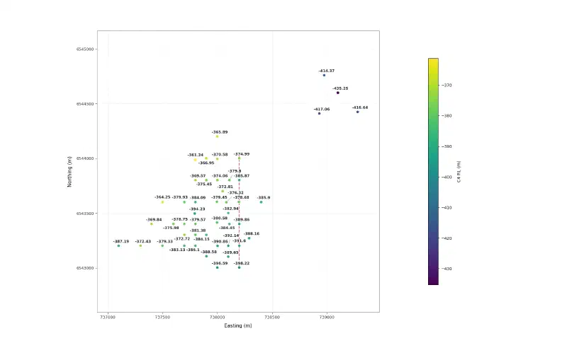
3. Draw c4_map.png at exactly 1800 x 1092 pixels: a plan view with equal axis scales in metres, each hole as a dot coloured by C4 RL with one colour bar, the RL value beside each dot without overlapping labels, and a dashed line along easting 738,200 from northing 6,543,000 to 6,544,050 for the section line of the previous guide. No figure title.
4. In your report, give the number of holes kept, the RL range of C4, and every hole where the pick differs from the stratigraphic log by more than 2 m, with the rows on either side of both depths.

Save the tables as CSV and the figure as PNG.
The agent kept 47 holes. It left out CAR001, which has no collar elevation, and CAR041, which is drilled at −60°. C4 ranges from RL −435.25 m to −361.24 m. We checked every pick against the source files, and they all match.
Seven picks differ from the stratigraphic log by more than 2 m:
| Hole | Our pick (m) | Stratigraphic log (m) | Difference (m) |
|---|---|---|---|
| CAR014 | 461.2 | 472.9 | −11.7 |
| CAR046 | 476.2 | 472.3 | +3.9 |
| CAR049 | 483.6 | 475.65 | +7.95 |
| CAR050 | 477.2 | 463.85 | +13.35 |
| CAR051 | 478.4 | 473.85 | +4.55 |
| CAR053 | 471.7 | 459.3 | +12.4 |
| CAR057 | 477.45 | 469.0 | +8.45 |
In six of them, the stratigraphic log starts the granite at the top of the last conglomerate. CAR014 is the opposite case: the rock log shows granite from 461.2 m, directly below conglomerate, but the stratigraphic log starts it 11.7 m deeper. Mixing these conventions would add steps of up to 13 m to the surface.
Step 2: Interpolate With Three Methods
Next, the agent estimates C4 on a 10 m grid with IDW, a thin plate spline and ordinary kriging. It then runs leave-one-out cross-validation: it hides one hole, predicts it from the other 46, and repeats for every hole.
Next, interpolate the C4 surface from c4_picks.csv. We are estimating the elevation of a geological boundary, not averaging rock types.

Grid: 10 m cells covering easting 737,000 to 739,400 and northing 6,542,900 to 6,544,900.

1. Interpolate C4 RL on the grid with three methods:
- IDW: inverse distance weighting with power 2, using all holes.
- RBF: a thin plate spline radial basis function that passes exactly through every hole.
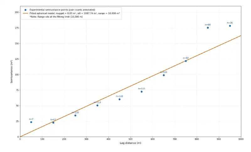
- Kriging: ordinary kriging. Compute the experimental semivariogram with 100 m lags up to 1,000 m, fit a spherical model, and report its nugget, sill and range. If the semivariogram keeps rising without levelling off, say so, because that points to a regional trend. Also save the kriging standard deviation.
Save each grid as CSV with easting, northing and rl, with the kriging standard deviation as a fourth column in the kriging grid.
2. Test each method with leave-one-out cross-validation: remove one hole, predict its C4 from the others, and repeat for every hole. Save loo_results.csv with hole, actual_rl, and the prediction and error (prediction minus actual) for each method. Report each method's mean error, root mean square error and largest error with its hole.
3. Draw c4_methods.png at exactly 1800 x 1092 pixels: three maps side by side, one per method, with the same colour scale for C4 RL, contours every 10 m, the holes as black dots, equal axis scales, plain tick labels in metres and a dashed line along easting 738,200 for the section line. Show cells more than 250 m from the nearest hole in light grey. Put each method name inside its map and one shared colour bar to the right. No figure title.
4. Draw c4_variogram.png with the experimental points at their lag centres, their pair counts, and the fitted model as a line with its nugget, sill and range in the legend. No figure title.

Report only values computed in code in this run. Save the tables as CSV and the figures as PNG.
The cross-validation results, in metres, where error is prediction minus actual:
| Method | Mean error | Root mean square error | Largest error |
|---|---|---|---|
| IDW | +0.65 | 7.33 | +28.13 (CAR011) |
| RBF | −0.72 | 8.52 | −34.92 (CAR036) |
| Kriging | −0.23 | 6.15 | +18.35 (CAR011) |
We reran all three tests ourselves. IDW and kriging match exactly, and our own thin plate spline gives a root mean square error of 8.47 m, a small difference from implementation details.
Each method’s largest error falls in the four north-eastern holes. That group has few neighbours, and CAR011, the deepest point in the area, sits in its middle. Once hidden, it can only be predicted from the shallower holes around it.
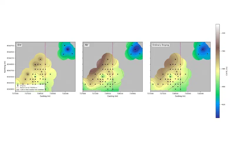
The maps show each method’s character:
- IDW draws bull’s-eyes around single holes, because each hole pulls the cells near it towards its own value.
- The thin plate spline stays smooth but swings beyond the data. In the north-west it reaches RL −349.5 m, about 12 m higher than any hole, even within 250 m of one.
- Kriging sits between the two and fits the holes exactly, because its fitted model has no nugget.
The semivariogram measures how different two points are on average at a given distance. Here it rises steadily to 850 m and shows no clear sill, the level where it would flatten, within 1,000 m. The fitted spherical model has a nugget of 0 m², a sill of 1,087.74 m² and a range of 10,000 m, which is the fitting limit. In practice, that model behaves like a straight line and hints at a regional trend, with C4 deepening to the north-east.
Step 3: Choose a Method and Map the Uncertainty
We chose ordinary kriging as the working surface, because it has the smallest cross-validation error. This prompt records that choice and maps where the surface is uncertain:
I compared the three methods as the geologist. I choose ordinary kriging as the working surface, because it has the smallest leave-one-out error (root mean square 6.15 m, largest 18.35 m at CAR011). Its variogram has not levelled off by 1,000 m, so its standard deviation depends on the fitted model and is a guide, not a guarantee.

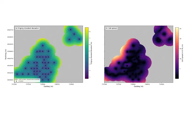
1. Draw c4_uncertainty.png at exactly 1800 x 1092 pixels with two maps side by side: the kriging standard deviation, and the spread between the three methods (highest minus lowest RL in each cell). Use the same 250 m grey mask, the holes as black dots, equal axis scales and plain tick labels. No figure title.
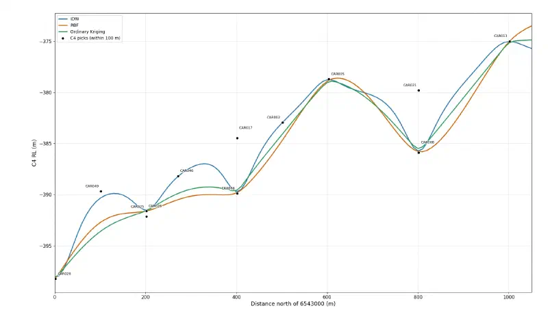
2. Draw c4_profile.png at exactly 1800 x 1092 pixels: the three surfaces sampled along easting 738,200 from northing 6,543,000 to 6,544,050, as RL against distance north of 6,543,000, with the C4 picks of the holes within 100 m of that line as labelled points. No figure title.
3. Report the share of the grid within 250 m of a hole, the largest method spread and kriging standard deviation inside that zone and outside it, and the largest gap between the kriging profile and the other two along the section line.

Report only values computed in code in this run. Save the figures as PNG.
The uncertainty depends mostly on the distance to the nearest hole:
| Measure | Within 250 m of a hole | Beyond 250 m |
|---|---|---|
| Share of the grid | 45.4% | 54.6% |
| Largest spread between methods | 25.6 m | 50.2 m |
| Largest kriging standard deviation | 8.65 m | 17.6 m |
We also calculated the median spread between the methods: 2.3 m within 100 m of a hole and 4.5 m within 250 m.
Along the section line from the previous guide, the holes are close together, so the three methods stay within about 3.3 m of each other. The profile also shows something a map hides: holes 90 to 100 m off the line, such as CAR017 and CAR021, do not sit on the curves. The surface changes sideways as well as along the line.
Step 4: Open the Surface in the Geocluster Map
Finally, save the working surface as a GeoTIFF, a georeferenced image file that map software can place on the ground:
Next, put the working surface into the Geocluster map. Save the ordinary kriging C4 surface as c4_kriging_rl.tif and its standard deviation as c4_kriging_std.tif: single-band float32 GeoTIFFs, north up, 10 m pixels, origin at the top-left corner of the grid, CRS EPSG:7853 (GDA2020 / MGA zone 53), and nodata for cells more than 250 m from the nearest hole. Read both files back and report their size, bounds, CRS, nodata value and value range.Both files are 240 × 200 pixels with 21,773 valid cells, and they use EPSG:7853. We read them back ourselves, and every value we checked matches the kriging grid.
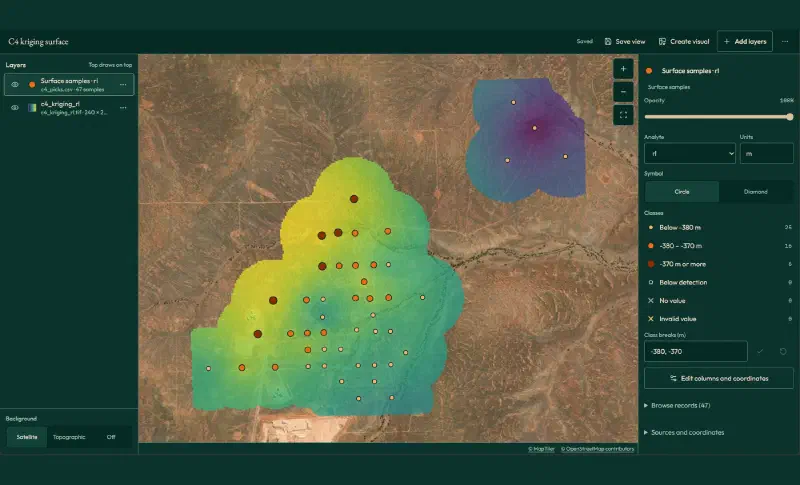
Then open Map in the top bar and add the two layers:
- Add layers, then Grids and images, then Add next to
c4_kriging_rl.tif. - Add layers, then Sample and drillhole tables, then Locate… next to
c4_picks.csv. - Under What the rows are, choose Surface samples. Set Sample ID to
hole, Assay value torl, Easting toeastingand Northing tonorthing. The coordinate system fills in as GDA2020 / MGA zone 53. Typemunder Units, then click Add to map. - Click the raster layer, pick the Viridis palette and lower its opacity so the satellite image shows through.
- Click Save view and give the map a name.
- Click Create visual to export the map as an image with a legend, a scale bar and a north arrow.
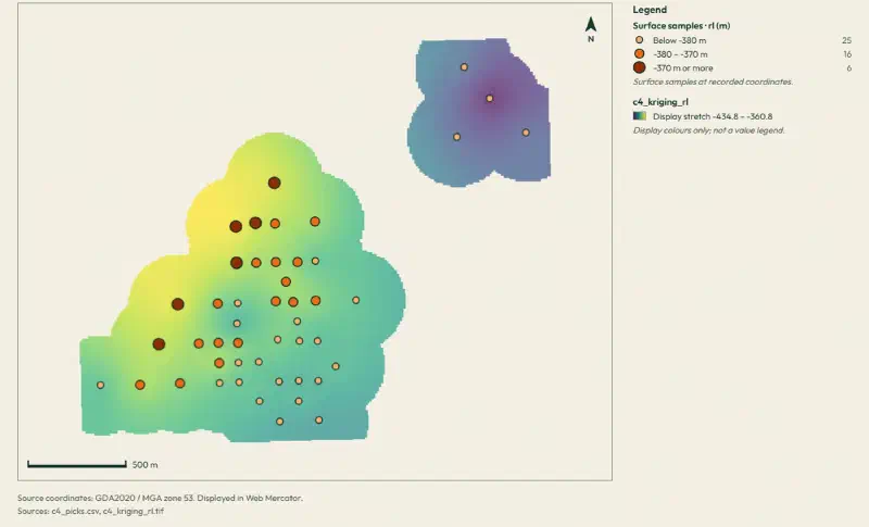
The 47 holes land exactly on the surface, including the four in the north-east. The map classes them as 25 holes below RL −380 m, 16 between −380 m and −370 m, and 6 above −370 m.
The exported visual is ready to drop into a report. Its colours are a display stretch from RL −434.8 m (purple) to −360.8 m (yellow), and Geocluster labels them as display colours, not a value legend. The values themselves stay in the GeoTIFF.
What the Interpolated Surface Shows
Read together, the four steps show what happens when you interpolate geological surfaces from real logs:
- A sloping basement. C4 lies highest, around RL −361 m, in the north-west of the main cluster and deepens to about RL −435 m in the north-east holes.
- A reliable core. Within 250 m of a hole, the median difference between the methods is 4.5 m.
- Thin control away from the holes. In the 840 m gap to the north-eastern holes, the methods differ by up to 16 m, and no hole tests them there. At the far north-western corner of the grid, 1.2 km from any hole, they differ by 50 m.
- No method wins everywhere. Kriging has the smallest errors here, but all three make their largest error in the same small group of four holes.
Limits When You Interpolate Geological Surfaces
When you interpolate geological surfaces from drillholes, the result carries these limits:
- Mathematics, not geology. None of the three methods knows about faults, folds or erosion. A fault between two holes would be smoothed into a slope.
- A model that has not settled. The semivariogram shows no clear sill within 1,000 m, so the kriging standard deviation depends on a model fitted at its limit. Read it as a guide.
- Masked does not mean known. Cells beyond 250 m are grey because nothing supports them, not because they are wrong.
- Picks first. The surface is only as good as the 47 picks under it, and seven of them depend on which logging convention you follow.
- One surface. A model with several surfaces must keep them in order, so they never cross. That is the job of a 3D geological model.
- Yearly updates. The SARIG package changes each year, so a later download may not match the numbers here, which come from the package sourced on 9 November 2026.
- Check the written summary. Treat the saved tables and figures as the result, and verify historical drilling data against its source. We recomputed the picks, the cross-validation and the GeoTIFF values from the source files.
FAQs
What does it mean to interpolate between boreholes?
It means estimating a value at places between drillholes from the values measured in them. For geological surfaces, the value is the elevation of a contact, such as the top of a rock unit. The result is a grid or map of that surface, which is only as reliable as the holes and the method behind it.
What is the difference between IDW and kriging?
IDW weights each hole by distance alone, so the nearest holes dominate and single holes form bull’s-eyes. Kriging first measures how the surface varies with distance in a variogram, then sets the weights from it and also estimates its own error. Kriging needs more setup, but it often predicts better and shows its uncertainty.
What is a variogram?
A variogram plots how different two measurements are on average against the distance between them. Close points are usually similar, and the difference grows with distance until it levels off at the sill. The distance where it levels off is the range. Kriging uses this curve to decide how much each hole should count.
Which interpolation method is best for geological surfaces?
No method is best everywhere. Test them on your own data with leave-one-out cross-validation, which hides each hole in turn and measures the prediction error. In this guide, ordinary kriging had the smallest error, but all three methods made their largest error in the same small group of four holes.
How far from a drillhole can you trust an interpolated surface?
It depends on how quickly the surface changes and how dense the holes are. Here, the median difference between the three methods was 4.5 m within 250 m of a hole, but they differed by up to 50 m farther away. Map the distance to the nearest hole and the spread between methods to see it.
Can you interpolate a contact that is cut by faults?
Not with a single smooth surface. IDW, splines and kriging all spread the offset across the space between holes. Split the area into fault blocks and interpolate each one separately, or use implicit modelling, which can include faults as surfaces. First check whether the contact really steps, as in a cross section.
Interpolate Surfaces in Geocluster
Open the Geocluster web workspace to interpolate geological surfaces in your browser, without writing code or setting up servers. Create a project, upload your area files (or your own contact picks), and send the four prompts above. You get three tested surfaces, an uncertainty map and a GeoTIFF layer in the Geocluster map.