TL;DR: Want to interpolate mineral grades between drillholes without writing code? Interpolating grades means estimating how much usable ore sits in the rock between the places a drill actually sampled. In the Geocluster workspace, six prompts to the built-in AI agent turn public gold results from 80 Western Australian drillholes into a 3D block model. The agent evens out the sample lengths, keeps the estimate inside the altered rock that carries the gold and limits a few extreme values. Then it compares two methods: inverse distance weighting, which simply trusts nearby samples more, and kriging, which first measures how far grades stay alike. On this data the simpler method did slightly better. You then open the blocks in 3D and on a map.
What Does It Mean to Interpolate Mineral Grades?
To interpolate mineral grades is to estimate a continuous value, such as grams of gold per tonne (g/t), at places no drillhole sampled, from the assays of nearby holes. You may see the same task written as grade interpolation between drillholes, or as interpolating drillhole assay data. It is one task in AI for geological modelling.
However, grades behave differently from the geological contacts of the previous guides. A contact is one surface; a grade changes from metre to metre, is often skewed by a few very rich samples, and runs farther in some directions than others. So grade interpolation adds steps of its own:
- Compositing: cut the assays into equal lengths, so every value carries the same weight.
- Domaining: estimate inside the rock that carries the metal, not across barren ground.
- Top cutting: cap a few extreme values, so one sample cannot inflate a large volume.
- Anisotropy: measure how far grades stay alike in each direction.
- Validation: check the estimates against holes the method did not see.
Part 1 of this series drew measured drill data in 3D cells with nothing interpolated. Here we estimate gold between the holes and compare IDW vs kriging, two common methods for the job.
Drillhole Data Used in This Guide
The data comes from open-file WAMEX report A114051, from Central Laverton in Western Australia. WAMEX is the state’s public archive of mineral exploration reports. We do not host a copy, so open the report page, go to the Document List tab and download drilling.zip.
Upload these five files from the archive to a new Geocluster project:
CL_WADL4_COLL2017A.txt: where each hole starts (the collars)CL_WADL4_SURV2017A.txt: direction readings down each holeCL_WADL4_GEOL2017A.txt: the geology logCL_WADL4_ASSAY2017A.txt: gold results from the labGeneric_Logging_Code2010.xls: the dictionary of logging codes
We use the 80 Goanna holes: the hole ID starts with GDDH and the collar north is between 6,813,600 and 6,814,400. Coordinates are in MGA zone 51 (EPSG:28351), in metres. These holes hold 5,127 gold assay rows: one is blank, and 1,360 are below the detection limit, written like <0.01.
The report describes what we are estimating. At Goanna, gold sits mostly in coarser sedimentary rock, in a zone about 5 m thick and up to 15 m thick. The zone follows a reverse fault that dips moderately east (the Granny Shear). The gold comes with strong silica, sericite and pyrite alteration, and the logs record that alteration as code ASMS (silica plus sericite).
How Do I Interpolate Mineral Grades Between Drillholes in Geocluster?
To interpolate mineral grades between drillholes, send six prompts one at a time in the same conversation, then load the result with the voxel wizard and the map. Wait until each prompt finishes, and keep the browser tab open while it runs.
Step 1: Convert the WAMEX Files to Tables
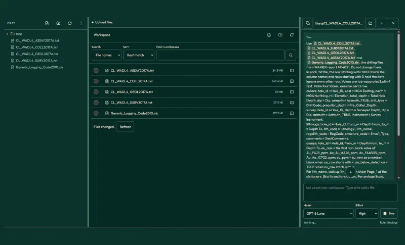
WAMEX text files are not plain tables. A row starting with H1000 holds the column names, rows starting with D hold the data, and rock codes need a lookup in a separate dictionary. So attach the five files with @ and paste this prompt:
Use @CL_WADL4_COLL2017A.txt, @CL_WADL4_SURV2017A.txt, @CL_WADL4_GEOL2017A.txt, @CL_WADL4_ASSAY2017A.txt and @Generic_Logging_Code2010.xls, the drilling files from WAMEX report A114051. Do not change them.
In each .txt file, the row starting with H1000 holds the column names and rows starting with D hold the data. Ignore every other row. Values are tab-separated Latin-1 text. Make four tables, one row per D row.
collars: hole_id = Hole_ID, east = MGA Easting, north = MGA Northing, rl = Elevation, total_depth = Total Hole Depth, dip = Dip, azimuth = Azimuth_TRUE, drill_type = Drill Code, precollar_depth = Pre_Collar_Depth.
survey: hole_id = Hole_ID, depth = Surveyed Depth, dip = Dip, azimuth = Azimuth_TRUE, instrument = Survey Instrument.
lithology: hole_id = Hole_id, from_m = Depth From, to_m = Depth To, lith_code = Lithology1, lith_name, regolith_code = RegCode, structure_code = Struc1_Type, comments = GeolComments.
assays: hole_id = Hole_id, from_m = Depth From, to_m = Depth To, au_raw = the first non-blank value of Au_FA25_ppm, Au_Au_AA26_ppm, Au_FAA505_ppm, Au_Au_ICP22_ppm; au_ppm = au_raw as a number, blank when au_raw starts with <; au_below_detection = TRUE when au_raw starts with <.
For lith_name, look up lith_code on sheet Page_1 of the dictionary. Skip its sections Colour, Percentage Scale, Lightness (Colour Intensity), Alteration and Regolith Processes, and Alteration Intensity, because the same code can mean something else there.
Keep the four tables as automatic outputs of this run and tell me where they are.
Report the rows and distinct hole_ids per table, every lith_code with no lith_name, the number of lithology rows with a blank lith_code and how many of those have a structure_code, and the lith_name of SAG, SAN, NATD and U.
The agent saved four tables, each covering all 1,805 holes in the archive:
| Table | Rows |
|---|---|
collars | 1,805 |
survey | 4,702 |
lithology | 25,842 |
assays | 71,238 |
We recomputed these counts from the raw files, and every assay row matches its source row. Three assay values are words rather than numbers (L.I.P once and SNR twice), so they stay blank, but none of them is in a Goanna hole.
Step 2: Composite the Gold Assays
Assays come in different lengths, from a few centimetres to several metres. A long sample should count for more than a short one. So before you interpolate mineral grades, composite them: cut each hole into 1 m pieces and give each piece the length-weighted grade of its assays.
Next, composite the gold assays of the Goanna holes. Use the collars, survey, lithology and assays tables from the conversion.

Goanna holes are holes whose hole_id starts with GDDH and whose collar north is between 6,813,600 and 6,814,400. Desurvey them with minimum curvature from the collar, using only survey rows with instrument GYRO_MEMS, EZYGYRO or ALIGNER, keeping the first row where a depth repeats, using the azimuths as they are, and continuing the last direction beyond the last kept station.

1. Composite the gold assays to 1 m down each hole, length-weighted, starting at the first assay of each hole. Use half the detection limit (the number after < in au_raw) for below-detection results and leave unsampled metres out. Round sampled_length_m to 0.001 m and drop composites with less than 0.5 m of sampled length. Give each composite hole_id, from_m, to_m, the east, north and z of its midpoint, au_ppm, sampled_length_m and the lith_name at its midpoint. Lithology rows with a blank lith_code are structure records (FLT, CAN and similar), not rock intervals, so leave them out of that lookup; where rock rows overlap, keep the first in file order.
2. Report the number of raw samples and composites, and for both the mean, median, 90th, 97.5th and 99th percentiles, maximum and coefficient of variation.
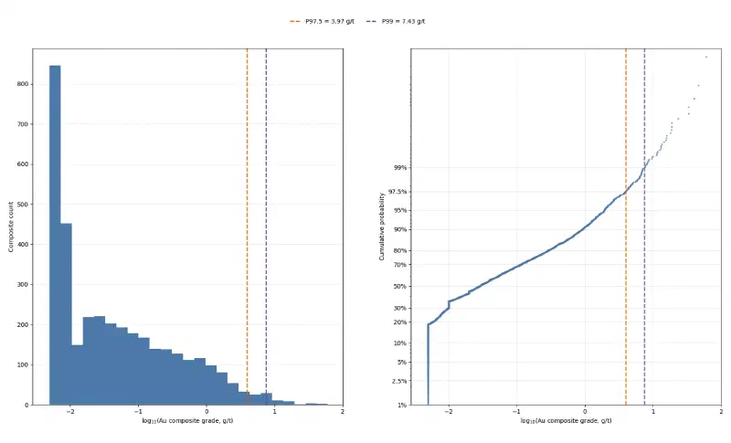
3. Draw au_distribution.png at exactly 1800 x 1092 pixels with a histogram of log10 composite grade and a log-probability plot, marking the 97.5th and 99th percentiles with their values in g/t to two decimals in the legend. No figure title and no footer note.
4. Report the mean composite grade and the share above 0.5 g/t for each lith_name with at least 20 composites.

Report only values computed in code in this run. Save the composites as CSV and the figure as PNG.
Compositing trims the extremes. The plain mean drops because short samples run richer, and each counts as one value. Assays under 0.5 m long average 0.90 g/t, those near 1 m only 0.20 g/t. Weighted by length, the raw assays average 0.470 g/t, almost the same as the composites.
| Statistic | Raw assays | 1 m composites |
|---|---|---|
| Count | 5,126 | 3,605 |
| Mean (g/t) | 0.555 | 0.467 |
| Median (g/t) | 0.030 | 0.029 |
| 97.5th percentile (g/t) | 4.19 | 3.97 |
| 99th percentile (g/t) | 10.84 | 7.43 |
| Maximum (g/t) | 93.1 | 59.92 |
| Coefficient of variation | 5.38 | 4.61 |
The coefficient of variation (CV, the standard deviation divided by the mean) stays above 4. That is typical of gold: most metres are nearly barren and a few are rich. In Arenite, the coarser sedimentary rock, composites average 0.68 g/t and 21.1% exceed 0.5 g/t; in Argillite, the finer one, they average 0.38 g/t and 12.1% exceed it. That fits the report.
Two rules in the prompt came from checking the first run:
- Structure rows are not rocks. Rows with no rock code record a fault (
FLT) or a contact (CAN). Without the rule, 66 composites took a blank rock name from them. - Round before you compare. A composite with exactly 0.5 m sampled came out as 0.49999 m in floating point and was dropped. Rounding keeps it.
Step 3: Build a Domain From the Logged Alteration
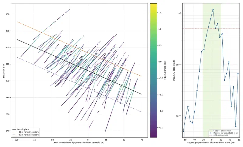
A domain is the volume you estimate in. If you interpolate mineral grades across everything, high grades leak into barren rock. Clustering can suggest a geological domain from the data, but here the geology already names one: the silica and sericite alteration around the shear. So we take the centre of the logged ASMS alteration in each hole and fit a plane through those centres. Then we keep every composite within a set distance of the plane.
Next, set up the estimation domain and the top cut. Use the composites from the previous step and the raw lithology file CL_WADL4_GEOL2017A.txt.

The A114051 report says Goanna gold sits in silica-sericite-pyrite alteration along the Granny Shear, a moderately east-dipping reverse fault. The logs record this alteration as ASMS (Silica + Sericite in the logging dictionary) in Alt1_Mineral or Alt2_Mineral.

1. For each Goanna hole, take the rows of CL_WADL4_GEOL2017A.txt with ASMS in Alt1_Mineral or Alt2_Mineral and a positive length. Find the length-weighted mean of their midpoint depths and desurvey that depth with the same method as the composites. Fit a least-squares plane z = a + b × east + c × north through these hole centres. Report the number of holes used, the dip and dip direction, and the spread of the perpendicular residuals.
2. Compute the perpendicular distance from every composite midpoint to the plane, positive above it. Report the number of composites, mean grade and share above 0.5 g/t in 5 m distance bins.
3. The domain is all composites within a half-width of the plane. Choose the smallest half-width of 10, 15, 20 or 25 m that holds at least 90% of the gold, measuring gold as au_ppm × sampled_length_m. Report the count, mean grade, share above 0.5 g/t and share of the gold inside and outside the domain, and the number of holes with a composite inside.
4. Draw domain_check.png at exactly 1800 x 1092 pixels with two panels. Left, about two thirds of the width: a cross section looking along strike, with distance along the dip direction on the horizontal axis and z on the vertical axis at equal scale, composites coloured by log10 grade, the plane as a solid line and the domain edges as dashed lines. Right: mean grade by 5 m distance bin with the domain shaded. Grades in g/t, no text in the panel corners and no figure title.
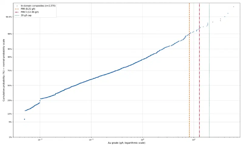
5. Inside the domain, draw topcut.png at exactly 1800 x 1092 pixels: a log-probability plot of the domain composites. For caps at the 99th and 99.5th percentiles and at the value where the upper tail breaks away from the trend, report the cap, the number of composites capped, the capped mean, the coefficient of variation before and after, and the share of the gold removed. Recommend one cap and say why. Mark the three caps on the plot. No figure title.

Report only values computed in code in this run. Save the composites with the distance and an in_domain column as CSV, the plane coefficients as CSV, and both figures as PNG under new file names.
Of the 80 holes, 66 log ASMS. The plane through their centres dips 20.8° toward 059°, east-north-east, the direction the report gives. The centres scatter around it with a standard deviation of 9.8 m. Grade peaks right at the plane, at 1.19 g/t in the first 5 m above it. More than 25 m from the plane, no 5 m bin averages over 0.12 g/t.
| Half-width | Composites inside | Gold inside |
|---|---|---|
| 10 m | 1,464 | 66.2% |
| 15 m | 2,089 | 84.6% |
| 20 m | 2,570 | 92.2% |
| 25 m | 2,909 | 98.2% |
As a result, the rule picks 20 m. Inside, 2,570 composites from all 80 holes average 0.604 g/t; the 1,035 outside average 0.129 g/t. The domain is wider than the 5 m to 15 m zone in the report because one plane cannot follow every bend of the shear.
Step 4: Choose a Top Cut
The agent offered three caps for the domain composites, and recommended the 99.5th percentile:
| Cap | Value (g/t) | Composites capped | Gold removed | CV after |
|---|---|---|---|---|
| Fitted break | 0.49 | 514 | 73.6% | 1.20 |
| 99th percentile | 8.21 | 26 | 18.0% | 2.56 |
| 99.5th percentile | 12.86 | 13 | 12.3% | 2.85 |
| Gap in the tail (our choice) | 20.00 | 6 | 7.7% | 3.17 |
However, we rejected all three. The fitted break marks where the main population bends, not where outliers start, and capping there would remove three quarters of the gold. The percentiles are only starting points. The plot itself shows a clear gap between 18.8 and 23.5 g/t with six composites above it, so we capped at 20 g/t. Your agent may fit a different break, so edit the numbers in the next prompt to match your plot. Keep the rule: cap at a gap in the tail and check how much gold it removes.
Step 5: Measure Anisotropy With Variograms
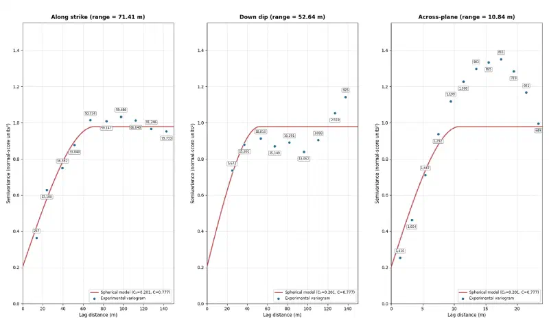
Anisotropy means grades stay alike over longer distances in some directions than in others. A variogram measures this: for pairs of samples at a growing distance apart, it plots half the mean squared difference in grade. Beyond the distance where the curve levels off, called the range, samples no longer help each other. Gold grades are so skewed that we compute variograms on normal scores (ranks turned into a bell curve), in three directions along the plane of the zone.
Decisions on the domain and the top cut:
- Keep the 20 m domain.
- Do not use the fitted break at 0.49 g/t. It marks a change of slope in the main population, not the upper tail, and capping there would remove 74% of the gold. Cap the domain composites at 20 g/t instead: the log-probability plot has a gap between 18.8 and 23.5 g/t, and only six composites sit above it. List those six composites (hole_id, from_m, au_ppm) and report the capped mean, the coefficient of variation and the share of the gold removed at 20 g/t.
- Redraw the top-cut plot from the uncapped domain grades as topcut_v2.png at the same size, marking P99, P99.5 and a line labelled "20 g/t cap", with grades in g/t, legend values to two decimals, the probability axis starting at 1%, no text box and no figure title.

Then study the continuity of the capped grades inside the domain.

1. Rotate the composite midpoints into the plane's frame: along strike (dip direction minus 90°), down dip within the plane, and across the plane.
2. Transform the capped domain grades to normal scores.
3. Compute experimental variograms of the normal scores in the three directions with an angular tolerance of 22.5°: along strike and down dip in 15 m classes up to 150 m, across the plane in 2 m classes up to 24 m. The classes start at 0: [0, lag), [lag, 2 × lag) and so on. Skip classes with fewer than 30 pairs and plot each class at the mean distance of its pairs.
4. Fit one spherical structure plus a nugget, shared by all three directions with its own range in each, by least squares weighted by the number of pairs. Report the nugget, the sill, the three ranges and the anisotropy ratios.
5. Draw variograms.png at exactly 1800 x 1092 pixels with three panels, one per direction, showing the experimental points with their pair counts and the fitted model line. No figure title.

Report only values computed in code in this run. Save the experimental variograms and the model as CSV, and every figure as PNG under a new file name.
The cap cuts the coefficient of variation from 4.09 to 3.17 and the mean of the domain composites from 0.604 to 0.558 g/t. The fitted variogram model has a nugget of 0.20 of a total sill of 0.98, about 21%, and these ranges:
| Direction | Range | Ratio to across |
|---|---|---|
| Along strike | 71.4 m | 6.6:1 |
| Down dip | 52.6 m | 4.9:1 |
| Across the plane | 10.8 m | 1:1 |
So gold runs farthest along the strike of the shear and only about 11 m across it, close to the zone thickness in the report. Down dip, the first class had only 10 pairs, so that range rests on pairs 15 m or more apart.
Step 6: Estimate the Blocks With IDW and Kriging
Now the two methods. Inverse distance weighting (IDW) gives each nearby composite a weight of one over its distance squared. Ordinary kriging picks the weights that the variogram says give the smallest error. To keep the comparison fair, both use the same neighbours, and both measure distance with the anisotropy, so 70 m along strike counts like 10 m across the plane.
Decisions on the variograms: keep the 20 g/t cap. For estimation, use the model rounded: nugget 20% of the sill, one spherical structure, ranges 70 m along strike, 50 m down dip and 10 m across the plane. Scale the sill to the variance of the capped domain composites.

Now estimate gold grades between the holes inside the domain, by ordinary kriging and by inverse distance weighting, and check both.

1. Build a block model of 10 m × 10 m × 5 m blocks (east, north, z) with its lower corner at east 443,100, north 6,813,580 and z 230, and 36 × 70 × 32 blocks. Keep blocks whose centre lies within 20 m of the plane and within 25 m of the nearest domain composite. Give each block x_index, y_index and z_index counted from 0 at the lower corner.
2. Estimate each kept block centre from the capped domain composites with both methods, using the same neighbours: a search ellipsoid aligned with the plane with radii of 1.5 times the ranges, at most 24 composites, at most 6 from one hole, and at least 4 composites from at least 2 holes (leave the block empty otherwise). Kriging uses the model above; inverse distance uses power 2 on the anisotropic distance (distances divided by the ranges). Report the number of blocks kept and estimated, and the number of negative kriging estimates (keep them as they are).
3. Also give each block the capped grade of its nearest domain composite. Report the mean block grade for kriging, inverse distance and nearest composite, and the number of blocks at or above 0.5 and 1 g/t for each.
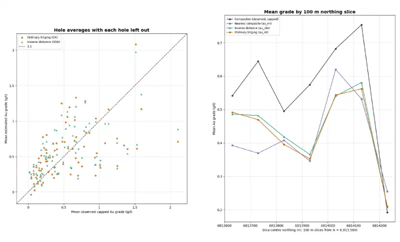
4. Leave-one-hole-out check: estimate every domain composite with both methods after removing its whole hole, with the same search. Report the mean error, RMSE, correlation and slope of the regression of true on estimated grade, for single composites and for the average of each hole.
5. Draw validation.png at exactly 1800 x 1092 pixels with two panels: left, hole averages of estimated against true grade for both methods with a 1:1 line; right, a swath plot of mean grade in 100 m northing slices from 6,813,580 for composites, nearest composite, inverse distance and kriging. Use the panel titles "Hole averages with each hole left out" and "Mean grade by 100 m northing slice", and show full coordinates without offset or scientific notation. No figure title.
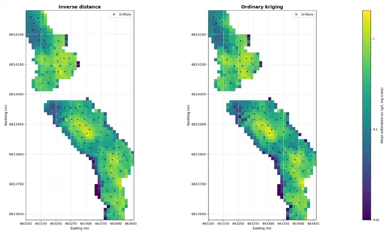
6. Draw grade_maps.png at exactly 1800 x 1092 pixels: two plan views side by side, titled "Inverse distance" and "Ordinary kriging", showing the mean block grade of each 10 m × 10 m column as a filled cell on one shared logarithmic colour scale in g/t starting at 0.01, with each hole marked at the mean position of its domain composites and labelled "Drillhole" in the legend. Show full coordinates without offset or scientific notation. No figure title.

Report only values computed in code in this run. Save the blocks as CSV with x_index, y_index, z_index, east, north, z, au_ok, au_idw and au_nn, the leave-one-hole-out results as CSV, and the figures as PNG under new file names.
The agent kept 6,026 blocks and estimated 6,025; one had too few neighbours. The nearest-composite grade works as a reference, because it reproduces the data without smoothing and without the extra weight of closely drilled ground.
| Method | Mean block grade (g/t) | Blocks at 0.5 g/t or more | Blocks at 1 g/t or more |
|---|---|---|---|
| Kriging | 0.424 | 1,370 | 820 |
| IDW | 0.436 | 1,480 | 856 |
| Nearest composite | 0.410 | 877 | 508 |
Overall, both methods land within 7% of the reference mean, well below the 0.558 g/t of the capped composites, which cluster where drilling and sampling are densest. Kriging also returned 238 negative grades, down to −1.20 g/t. Negative weights do that when nearby samples screen each other; IDW weights are always positive, so IDW cannot go below zero.
In the leave-one-hole-out check, the agent removes a whole hole and estimates its composites from the other holes:
| Scale | Method | RMSE (g/t) | Correlation | Slope |
|---|---|---|---|---|
| Single composite | Kriging | 1.779 | 0.211 | 0.471 |
| Single composite | IDW | 1.756 | 0.226 | 0.541 |
| Hole average | Kriging | 0.397 | 0.502 | 0.612 |
| Hole average | IDW | 0.374 | 0.550 | 0.704 |
A slope of 1 would mean no conditional bias; below 1, high estimates come out too high and low ones too low. At both scales IDW had the lower error, the higher correlation and the slope closer to 1. In our own recomputation, kriging with a nugget of up to 50% of the sill still did not beat IDW for single composites.
Step 7: Export the Grade Model
The last prompt records the choice and writes the files Geocluster loads: a block table for the voxel wizard, a GeoTIFF for the map, and one point per hole.
Decision on the estimates: use inverse distance for the final grade model. It did slightly better than kriging in the leave-one-hole-out check at both scales and gives no negative grades. Keep the kriging column for comparison.

1. Save goanna_grade_voxel.csv for Geocluster's Create voxel with only x_index, y_index, z_index, au_idw and au_ok, one row per estimated block.
2. Build goanna_idw_column_mean.tif from those blocks: for each x_index and y_index, the mean au_idw of the column's blocks. The grid has 36 columns (x_index 0 to 35, west to east) and 70 rows (row 0 is y_index 69, the north edge). Write a single-band float32 GeoTIFF in EPSG:28351 with nodata -9999 and the transform rasterio.transform.from_origin(443100, 6814280, 10, 10). Read it back and report the transform as a, b, c, d, e, f, the bounds (they must be 443100, 6813580, 443460, 6814280), and the number of valid pixels with their minimum, maximum and mean.
3. Save goanna_hole_grades.csv with hole_id, east, north (the mean position of the hole's domain composites), au_ppm (the mean of the capped grades of the hole's domain composites) and unit "g/t".

Report only values computed in code in this run. Save every file under the new name given.
The block table has 6,025 rows. The GeoTIFF has 830 filled 10 m cells, with column means from 0.005 to 2.05 g/t, and the hole table has 80 rows, led by GDDH0101 at 2.11 g/t.
Also, read the bounds back every time. Our first GeoTIFF had the six transform numbers in the wrong order, so a pixel claimed to be 443,100 m wide. The map refused it with “These coordinates fall outside the chosen coordinate system”. If the agent answers that it has no raster tool, ask it to hand the task to its Extended agent, which may install a raster library.
Step 8: Load the Grade Blocks in 3D
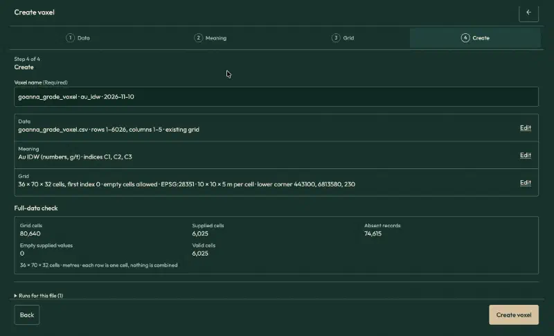
Open goanna_grade_voxel.csv, click Create voxel and fill in the wizard:
| Setting | Value |
|---|---|
| Table meaning | Existing grid |
| Header rows | 1, whole table |
| Value | au_idw, field name Au IDW, Numbers, unit g/t |
| Index X, Y, Z | x_index, y_index, z_index |
| Cells along X, Y, Z | 36, 70, 32 |
| First index | 0 |
| Empty cells | Allow empty cells |
| Coordinates | Physical coordinates, metres, Projected CRS |
| CRS | EPSG:28351 |
| Elevation reference | Collar RL, WAMEX A114051 |
| Lower corner X, Y, Z | 443100, 6813580, 230 |
| Cell size X, Y, Z | 10, 10, 5 |
Three settings need care:
- The confirmation box. On the Meaning page, tick “These columns hold the cell indices and value for every selected row”, or the wizard will not continue.
- Cells along Z. Type 32. “Suggest from data” sizes the grid from the largest index on each axis, which drops the empty layers above the highest block.
- Elevation reference. The collar file gives its vertical datum as “Nominal”, so do not call it AHD.
The full-data check reports 80,640 grid cells, 6,025 supplied and valid, and 74,615 absent, which become empty cells.
Step 9: View and Slice the Grade Blocks
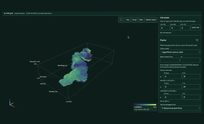
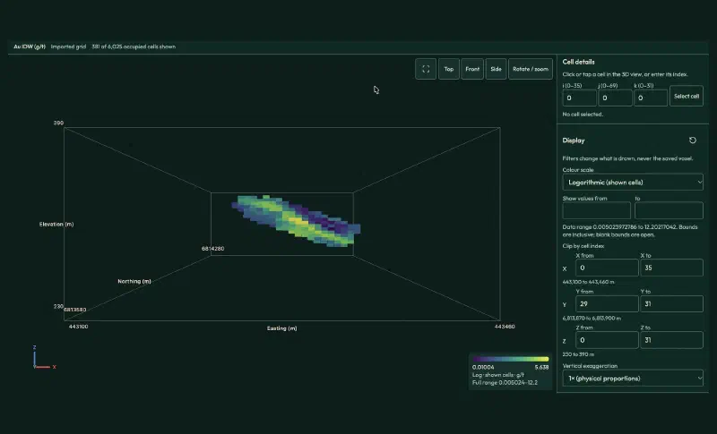
Click Create voxel and open it in 3D. Set Colour scale to Logarithmic (shown cells). On a linear scale, the few blocks near 12 g/t stretch the colours, so nearly every block looks the same dark purple.
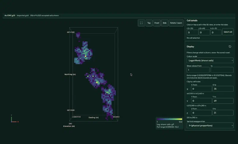
To see only the better ground, type 1 in Show values from and leave to blank, then click Top. The viewer then shows 856 blocks at 1 g/t or more, in three groups along the trend: at this cut-off the southern pod splits in two.
For a slice across the zone, clear the value filter, set Y from 29 to 31 (northing 6,813,870 to 6,813,900 m) and click Front. The 381 blocks of this slice dip east, from about RL 340 m in the west to about RL 295 m in the east. The richest blocks sit in the middle of the zone.
Step 10: Map the Grade Model
Open Map, click Add layers, choose Grids and images and add goanna_idw_column_mean.tif, with the Viridis colours. Then open Sample and drillhole tables, click Locate… on goanna_hole_grades.csv and fill in:
- What the rows are: Surface samples, the option for one point per row.
- Sample ID, Assay value, Easting, Northing:
hole_id,au_ppm,east,north. - Qualifier column: leave it empty. It is for detection flags such as
<, not for units. - Coordinate system and Units: GDA94 / MGA zone 51, and
g/tin place of theppmit reads from the column name.
On a satellite background, the blocks sit along the eastern wall of an open pit. That fits the report, which describes this program as infill drilling on the eastern side of the Goanna deposit.
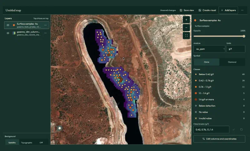
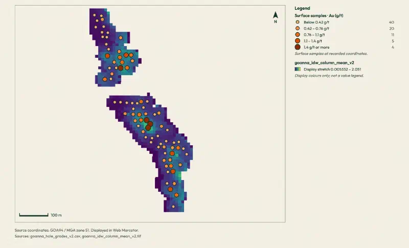
For a clean figure, click Create visual. It leaves out the satellite background and starts from the current view. Fit to layers stops at a fixed zoom, which leaves this small area tiny, so zoom in on the main map first and skip that button.
IDW vs Kriging: What the Comparison Shows
Read together, the steps show what it takes to interpolate mineral grades on this deposit:
- The domain mattered most. One plane through the logged alteration holds 92% of the gold in a slab 40 m thick, and the grade outside it averages 0.13 g/t.
- The cap was a judgement call. The automatic break would have removed 74% of the gold; the gap in the tail removed 7.7%.
- IDW edged out kriging. IDW had lower errors and less conditional bias at both scales, and no negative grades.
- Both methods agree on the picture. Two pods of higher grade along a north-north-west trend, inside a zone that dips east.
Still, kriging is not worse in general. With 1 m gold composites, a 21% nugget and a narrow zone, distance alone probably carried most of the information. A geologist would tune the search, test a finer domain and compare again before choosing.
Limits When You Interpolate Mineral Grades This Way
The result of this workflow carries these limits:
- One plane for the domain. The shear bends, so a 40 m slab holds low-grade margins along with the 5 m to 15 m zone. A wireframe that follows the zone hole by hole would be tighter.
- Logged alteration. Fourteen holes log no
ASMS, so the plane rests on 66 holes and on how each geologist logged. - Point estimates. Each block takes the grade estimated at its centre, not the average over the block. So the blocks vary more than true 10 m by 10 m by 5 m blocks would.
- Weak at the metre scale. A correlation near 0.2 for single composites means neither method predicts an individual metre well. Hole averages are far better.
- A screening model, not a resource. The 1 g/t blocks show where gold concentrates; they are not tonnes and grade you could report.
- Map placement. Geocluster converts the GDA94 coordinates to the web map with a stated accuracy of about 3 m, fine for 10 m cells.
- Check the written summary. One report listed six capped grades that did not match the file. So treat the saved tables and figures as the result, and verify historical drilling data against its source. We recomputed the composites, the domain, the variograms, the estimates and the exported files from the raw WAMEX files.
FAQs
Is kriging always better than IDW for mineral grades?
No. Kriging is optimal only when its variogram model fits the data well. In this guide, IDW gave slightly lower errors and less conditional bias in a leave-one-hole-out check, and kriging produced negative grades. Compare both methods on your own data, with the same neighbours, before you choose one.
Why composite drillhole assays before interpolating?
Assays come in different lengths, and a long sample says more about the rock than a short one. Compositing cuts each hole into equal lengths, such as 1 m, and gives each piece a length-weighted grade. Every value then carries the same support, so averages, variograms and estimates are not distorted by sample length.
How do you choose a top cut for gold grades?
Start with a log-probability plot of the composites in one domain. Look for a break or a gap in the upper tail, where a few values leave the trend. Then check how much metal each candidate cap removes. Percentiles and automatic breaks are starting points, not answers.
Why estimate grades inside a geological domain?
Grades in different rocks or structures belong to different populations. If you interpolate across a domain boundary, high grades spread into barren rock and low grades dilute the mineralised zone. A domain, here a slab around the logged alteration, keeps each estimate among samples from the same geological setting.
What is anisotropy in grade interpolation?
Anisotropy means grades stay alike over longer distances in some directions than in others. At Goanna, grades stay alike for about 71 m along the strike of the shear, but only about 11 m across it. An anisotropic search gives samples along the zone more weight than samples at the same distance across it.
How do you check a grade model against drillholes?
Remove one hole at a time, estimate its samples from the remaining holes, and compare estimates with true grades. Report the error, the correlation and the regression slope, for single samples and for hole averages. Swath plots by slice and a comparison with nearest-sample grades show whether the model keeps the mean.
Interpolate Mineral Grades in Geocluster
Open the Geocluster web workspace to interpolate mineral grades between drillholes in your browser, without writing code or setting up servers. Upload the five WAMEX files (or your own logs and assays), send the six prompts above, and load the result with the voxel wizard and the map. You get composites, a domain, a checked comparison of IDW and kriging, and a grade model you can slice in 3D.