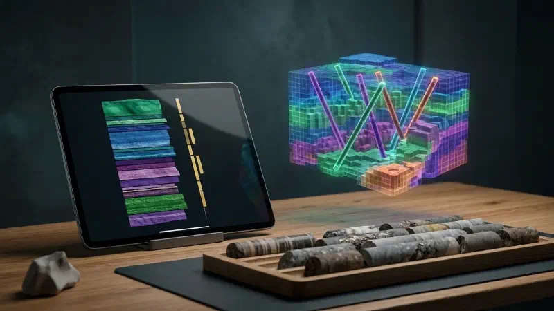
TL;DR: Want to visualise lithology from drillhole logs without writing code? In the Geocluster workspace, four prompts to the built-in AI agent and one short wizard turn public drilling files into clean tables and three views. A strip log draws one hole as a column. A cross-section draws several holes on one slice of ground. A voxel model sorts the rock types into a 3D grid of cells. Nothing is guessed between holes, so this comes before any interpretation of how rock units connect. We show every step on 80 real holes from a public Western Australian report.
What Does It Mean to Visualise Lithology From Drillhole Logs?
A drillhole log is the depth-by-depth record of one hole: rock type, weathering, structures and lab results. To visualise lithology from drillhole logs, you draw those records at the true position and depth of each hole. It is an early stage of geological modelling and estimation, done before anyone connects the ground between holes.
Each view answers a different question:
- Strip log: what did one hole pass through, and how does gold line up with the rock?
- Cross-section: how do neighbouring holes compare on one slice of ground?
- Voxel model: where do the rock types sit in 3D?
Part 1 of this series used vertical holes and gold grades only. Unlike that first guide, this part uses inclined holes with rock types.
Every view still shows measured intervals and leaves unsampled ground empty. A finished geological cross section also interprets the ground between holes, and that belongs to a later part.
Drillhole Data Used in This Guide
The data comes from open-file WAMEX report A114051, from Central Laverton in Western Australia. WAMEX is the state’s public archive of mineral exploration reports. We do not host a copy, so open the report page, go to the Document List tab and download drilling.zip.
Upload these five files from the archive to a new Geocluster project:
CL_WADL4_COLL2017A.txt: where each hole starts (the collars)CL_WADL4_SURV2017A.txt: direction readings down each holeCL_WADL4_GEOL2017A.txt: the geology logCL_WADL4_ASSAY2017A.txt: gold results from the labGeneric_Logging_Code2010.xls: the dictionary of logging codes
Four things about this data shape the steps below:
- 1,805 holes in total. Coordinates are in MGA zone 51 (EPSG:28351), in metres.
- 80 holes are used for the views. We call them the Goanna holes: the hole ID starts with GDDH and the collar north is between 6,813,600 and 6,814,400.
- The upper part of many holes has no rock record. In GDDH0060, the first 89.1 m were drilled without logging.
- Some rows are not rocks. Of the 25,842 geology rows, 1,475 have no rock code. They describe a fault, a shear or a contact instead.
How Do I Visualise Lithology From Drillhole Logs in Geocluster?
To visualise lithology from drillhole logs, start with four prompts to the agent. Send them one at a time in the same conversation, and wait until each one finishes. After that, only the voxel wizard is manual.
Step 1: Convert the WAMEX Drillhole Logs to Tables
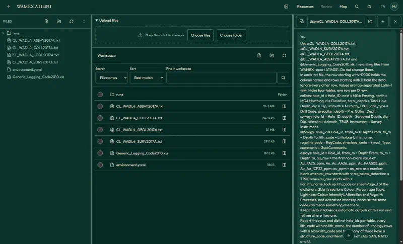
WAMEX text files are not plain tables. A row starting with H1000 holds the column names, rows starting with D hold the data, and rock codes need a lookup in a separate dictionary. So attach the five files with @ and paste this prompt:
Use @CL_WADL4_COLL2017A.txt, @CL_WADL4_SURV2017A.txt, @CL_WADL4_GEOL2017A.txt, @CL_WADL4_ASSAY2017A.txt and @Generic_Logging_Code2010.xls, the drilling files from WAMEX report A114051. Do not change them.
In each .txt file, the row starting with H1000 holds the column names and rows starting with D hold the data. Ignore every other row. Values are tab-separated Latin-1 text. Make four tables, one row per D row.
collars: hole_id = Hole_ID, east = MGA Easting, north = MGA Northing, rl = Elevation, total_depth = Total Hole Depth, dip = Dip, azimuth = Azimuth_TRUE, drill_type = Drill Code, precollar_depth = Pre_Collar_Depth.
survey: hole_id = Hole_ID, depth = Surveyed Depth, dip = Dip, azimuth = Azimuth_TRUE, instrument = Survey Instrument.
lithology: hole_id = Hole_id, from_m = Depth From, to_m = Depth To, lith_code = Lithology1, lith_name, regolith_code = RegCode, structure_code = Struc1_Type, comments = GeolComments.
assays: hole_id = Hole_id, from_m = Depth From, to_m = Depth To, au_raw = the first non-blank value of Au_FA25_ppm, Au_Au_AA26_ppm, Au_FAA505_ppm, Au_Au_ICP22_ppm; au_ppm = au_raw as a number, blank when au_raw starts with <; au_below_detection = TRUE when au_raw starts with <.
For lith_name, look up lith_code on sheet Page_1 of the dictionary. Skip its sections Colour, Percentage Scale, Lightness (Colour Intensity), Alteration and Regolith Processes, and Alteration Intensity, because the same code can mean something else there.
Keep the four tables as automatic outputs of this run and tell me where they are.
Report the rows and distinct hole_ids per table, every lith_code with no lith_name, the number of lithology rows with a blank lith_code and how many of those have a structure_code, and the lith_name of SAG, SAN, NATD and U.
The agent saved four tables, each covering all 1,805 holes:
| Table | Rows |
|---|---|
collars | 1,805 |
survey | 4,702 |
lithology | 25,842 |
assays | 71,238 |
We recomputed these counts from the raw files and they match. Only one code, FI (a single row outside the Goanna holes), has no dictionary name. Three assay values are words rather than numbers (L.I.P once and SNR twice), so they stay blank.
Step 2: Draw a Drillhole Lithology Strip Log
First, start with one hole. GDDH0060 has rock types, weathering codes, structures and a high-grade gold interval, so it fills every column. This prompt combines our first request with two follow-ups that set the size, colours and labels:
Use the collars, lithology and assays tables from the previous step. Rows with a blank lith_code are structure records, not rock intervals, so never draw them as rock. NPRC and NLST are No data.
Draw a downhole strip log of hole GDDH0060 as one figure, at exactly 1800 × 1092 pixels, with three columns sharing the depth axis, depth increasing downward from 0 to total depth, and all legends in one block to the right:
1. Lithology coloured by lith_name: Arenite #2F6DB5, Argillite #4DB97C, Altered Rock - Protolith Unrecognisable #7F5FD5, Granite #3D3D3D, No data #D9D9D9.
2. Regolith by regolith_code, no fill where blank: "RSPL (Lower saprolite)" #E377C2, "RSPR (Saprock)" #17BECF.
3. Gold: au_ppm as a horizontal bar for each assay interval on a log scale. Mark rows with au_below_detection TRUE with a hollow tick at the left edge, not as zero. Leave depths with no assay row blank. Label gaps "not sampled" at the right edge of the column with no background box, so the label covers no bar, and leave out the label for the 0.1 m gap at 143.6 to 143.7 m on this full-depth figure.
Draw each structure record as a short tick at its from_m and label only FLT and SH, each on a small white box to the right of its tick. Spread the three labels apart vertically and join each to its tick with a thin leader line. In the legend, write "FLT (Fault)" and "SH (Shear)".
Then draw a second figure with the same layout for 140 to 152 m only.
Do not open or view any image. Do not print file paths on any figure. Tell me where both figures are.
Report metres per lith_name, metres of No data, the first and last assay depth, the number of assay rows and of below-detection rows, the highest au_ppm with its interval, and the depth of each FLT and SH tick.
For GDDH0060, which is 171.46 m deep, the agent reported:
- Rock types: Argillite 38.12 m, Arenite 30.78 m, altered rock 8.50 m and granite 1.11 m.
- No data: 92.95 m, almost all of it above 89.1 m.
- Gold: 46 assay rows from 135 to 168.7 m. Eight are below detection and appear as hollow markers.
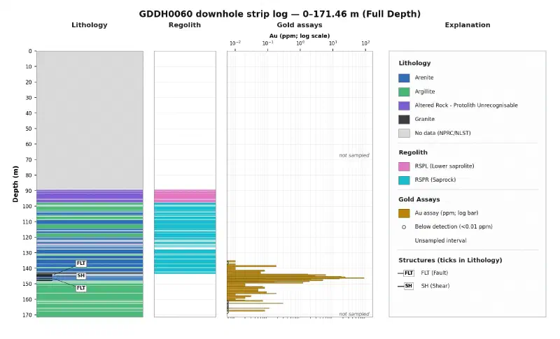
Weathering also has its own column. Lower saprolite (RSPL, 8.00 m) passes into saprock (RSPR, 41.65 m), and the code stops at 143.6 m.
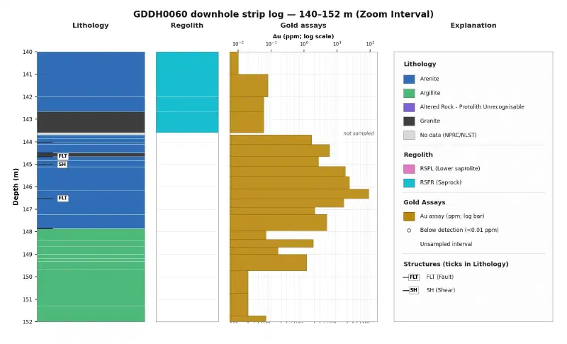
Meanwhile, the 12 m zoom shows what the full log compresses. For example, the highest gold result, 90.5 ppm from 146.10 to 146.52 m, ends at a logged fault. Two faults (144.66 m and 146.52 m) and a shear (145.02 m) all sit in Arenite, inside the gold interval.
Step 3: Compare Drillhole Lithology on a Cross-Section
A section needs each hole’s true path. Desurveying turns depth and direction readings into positions, so the choice of readings matters.
However, some holes carry both gyroscope readings and magnetic Reflex readings, and magnetic rock can disturb the second kind. In GDDH0057, the Reflex reading at 108 m gives an azimuth of 196.5°, while the gyroscope gives about 266° at 100 m and 110 m. That reading would put a false bend in the hole, so the prompt keeps only gyroscope and aligner readings.
The figure also marks gold composites. A composite merges neighbouring samples above a cut-off grade into one interval with a length-weighted average. This prompt combines our first request with one follow-up on trace lines, colours and labels:
Use the collars, survey, lithology and assays tables from the previous steps.
Rows with a blank lith_code are structure records, not rock intervals, so never draw them as rock. NPRC and NLST are No data. So is the GDDH0058 row from 0 to 89.4 m, because its comment reads "PCD precollar to 89.4m."
Goanna holes are holes whose hole_id starts with GDDH and whose collar north is between 6,813,600 and 6,814,400.
Geometry: minimum curvature starting at the collar. Use only survey rows with instrument GYRO_MEMS, EZYGYRO or ALIGNER. If a depth still appears twice in a hole, keep the first row. Use the azimuth values as they are, with no grid conversion. Beyond the last kept station, continue in the last direction.
Draw a vertical cross-section of the Goanna holes, looking north (west on the left, east on the right), and save a composite table.
Section line: northing 6,814,075, swath ±25 m. Use only holes with at least half of their desurveyed trace inside the swath.
Axes: horizontal = easting (m), 443,100 to 443,350; vertical = elevation (m RL) = collar rl minus vertical depth, 260 to 440. True scale 1:1, no vertical exaggeration. Scale bar, light grid, axis labels with units. Save at exactly 1800 × 1092 pixels, with the legend blocks to the right of the section.
Topography: a thin line through the collar points. Collar labels: hole_id inside the frame with a short leader line to the collar; holes on the same pad stacked without overlap.
Traces: per hole draw one trace line, black for each depth interval that has an assay row and thin grey for every depth with no assay row, including the upper part of each hole. Draw the part beyond the last kept survey station dashed. Add a narrow lithology strip on one side and a narrower regolith strip on the other side.
Lithology: colour by lith_name, with No data as one class "No data / precollar". Compute shares on the remaining logged length; keep Banded Iron Formation as its own class even under 2%; put every other name under 2% into "Other". Colours: Arenite #2F6DB5, Argillite #4DB97C, Altered Rock - Protolith Unrecognisable #7F5FD5, Banded Iron Formation #D4A017, Other #6B7C93, No data / precollar #D9D9D9. Red is for gold only.
Regolith: RSPU #8C5A2B, RSPL #E377C2, RSPR #17BECF, with their own legend block; no fill where regolith_code is blank.
Structure: draw only FLT and SH, each as one short tick across the trace at its from_m. Where ticks on one hole are within 3 m of each other, draw one combined label such as "2 FLT, 2 SH". Put every FLT or SH label on a small white box in empty space with a thin leader line.
Gold: composite au_ppm with cut-off 0.5 g/t, minimum length 2 m, and at most 2 m of consecutive material below cut-off inside a composite (an unsampled gap counts as below cut-off). Rows with blank au_ppm count as 0 g/t. A composite starts and ends on a sample at or above cut-off. Draw each composite as a red bar beside the trace, labelled "HOLE: X.XX m @ Y.YY g/t from Z.ZZ m" (two decimals), with a thin leader line to its own bar. Put the labels for GDDH0059 and both GDDH0061 composites in the empty area west of the traces, and the other five in a neat column east of easting 443,270 and below 340 m RL. Do not label single samples.
Do not draw anything between holes.
Do not open or view any image. In the plotting code, compute each label's bounding box, test it against every trace, strip, bar and other label, and move it until nothing touches. Do not print file paths on the figure. Tell me where the figure and the composite table are.
Report the holes used and excluded with the reason, the survey rows left out per hole, the metres beyond the last kept station per hole, the lithology classes with their share of logged length, the number of FLT and SH ticks, and the composite table.
The agent reported:
- Holes: seven used. GDDH0091 is out because only about 24% of its path falls inside the 50 m wide strip.
- Survey rows left out: 14 Reflex rows each in GDDH0057 and GDDH0059, 12 in GDDH0061, and one collar row per hole.
- Beyond the last survey station: 0.18 to 15.14 m per hole, drawn dashed.
- Rock shares of 429.09 m logged: Arenite 46.8%, Argillite 46.7%, altered rock 2.8%, banded iron formation 1.6% and other 2.2%.
- Structures: six faults and three shears.
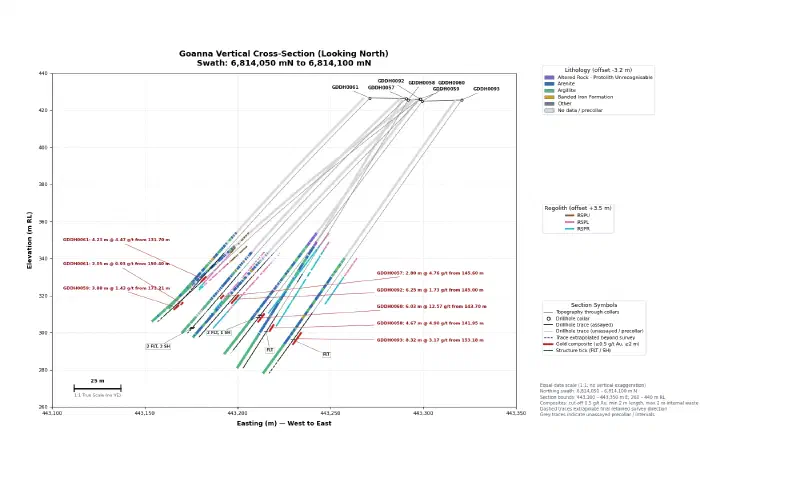
The eight composites match our own calculation from the raw files:
| Hole | From (m) | To (m) | Length (m) | Au (g/t) |
|---|---|---|---|---|
| GDDH0057 | 145.60 | 148.40 | 2.80 | 4.76 |
| GDDH0058 | 141.95 | 146.62 | 4.67 | 4.90 |
| GDDH0059 | 172.21 | 176.09 | 3.88 | 1.43 |
| GDDH0060 | 143.70 | 149.73 | 6.03 | 12.57 |
| GDDH0061 | 131.70 | 135.93 | 4.23 | 4.47 |
| GDDH0061 | 150.40 | 152.45 | 2.05 | 0.93 |
| GDDH0092 | 145.00 | 151.25 | 6.25 | 1.73 |
| GDDH0093 | 153.18 | 161.50 | 8.32 | 3.17 |
Step 4: Make the 3D Lithology Table
A voxel is a 3D cell, like a pixel in 3D. Because the builder needs one row per interval with a start point, an end point and a rock label, this prompt makes that table:
Use the collars, survey and lithology tables from the previous steps.
Rows with a blank lith_code are structure records, not rock intervals, so leave them out. NPRC and NLST are No data. So is the GDDH0058 row from 0 to 89.4 m, because its comment reads "PCD precollar to 89.4m."
Goanna holes are holes whose hole_id starts with GDDH and whose collar north is between 6,813,600 and 6,814,400.
Geometry: minimum curvature starting at the collar. Use only survey rows with instrument GYRO_MEMS, EZYGYRO or ALIGNER. If a depth still appears twice in a hole, keep the first row. Use the azimuth values as they are, with no grid conversion. Beyond the last kept station, continue in the last direction.
Make one table of the Goanna holes with one row per lithology row that has a lith_code. Columns: hole_id, from_m, to_m, start_east, start_north, start_z, end_east, end_north, end_z, rock_group. z is elevation in m RL (collar rl minus vertical depth).
Rows that are No data under the rules above, and rows with a blank lith_name, get rock_group No data. Otherwise use these labels exactly, by lith_code: SAG = Argillite; SAN = Arenite; NATD = Altered rock (protolith unknown); SMP = Conglomerate; SIF = Iron formation; S = Undifferentiated sediment; every other code = Minor rock types.
Do not open or view any image in this run. Keep the table as an automatic output of this run and tell me where it is.
Report the number of holes, rows per rock_group, survey rows left out per instrument, and the five longest extrapolations. Report only values computed in code in this run.
The table has 5,695 rows from 80 holes. The 309 structure rows stay out, and 693 survey rows also go unused (594 Reflex, 67 collar and 32 camera). We compared every row with the raw files: all labels match and the coordinates agree within 7 cm.
rock_group | Rows |
|---|---|
| Argillite | 2,348 |
| Arenite | 1,525 |
| No data | 1,049 |
| Minor rock types | 264 |
| Iron formation | 216 |
| Conglomerate | 134 |
| Undifferentiated sediment | 94 |
| Altered rock (protolith unknown) | 65 |
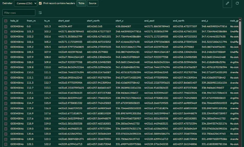
Step 5: Build the 3D Voxel Model
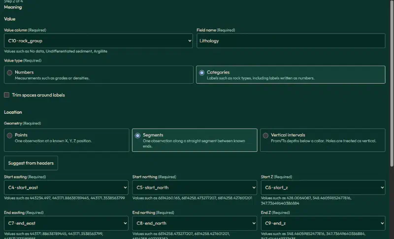
Then open the saved table, tick First record contains headers, and click Create voxel. The wizard has four steps: Data, Meaning, Grid and Create. Use these settings:
| Setting | Value |
|---|---|
| Table meaning | Observations |
| Header rows | 1 |
| Value | rock_group, name Lithology, Categories |
| Geometry | Segments |
| Start easting, northing, Z | start_east, start_north, start_z |
| End easting, northing, Z | end_east, end_north, end_z |
| Z values | Elevation, positive up |
| Coordinates | Projected CRS, EPSG:28351, metres |
| Elevation reference | Collar RL, WAMEX A114051 |
| Cell size | 5 × 5 × 5 m |
| Combining values | Longest total length per cell |
| Extent | Fit all accepted data |
| Missing values | No data |
Two settings are easy to miss:
- Missing values sits inside Source number format and missing values on the Grid step. Otherwise, empty intervals would become a rock class.
- The confirmation box at the end of the Meaning step is required before you continue.
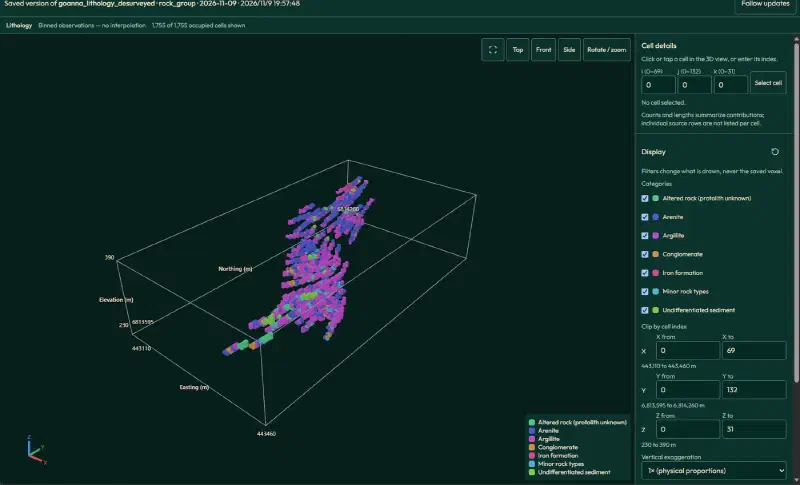
The wizard’s Create step runs a full-data check before anything is saved. It read 5,695 rows and accepted 4,646. The other 1,049 are the No data rows. The grid is 70 × 133 × 32 cells (297,920 in total), and 1,755 hold a rock type.
The wizard also offers a suggested cell size of 10 × 10 × 0.5 m. We leave it alone so the cells stay cubic.
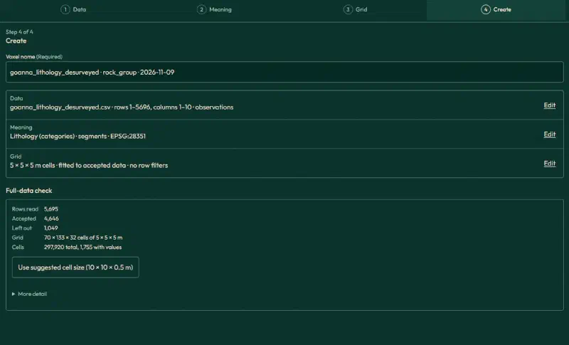
Then click Create voxel, wait until it finishes, and open it in 3D.
Step 6: Slice and Check the Lithology Model
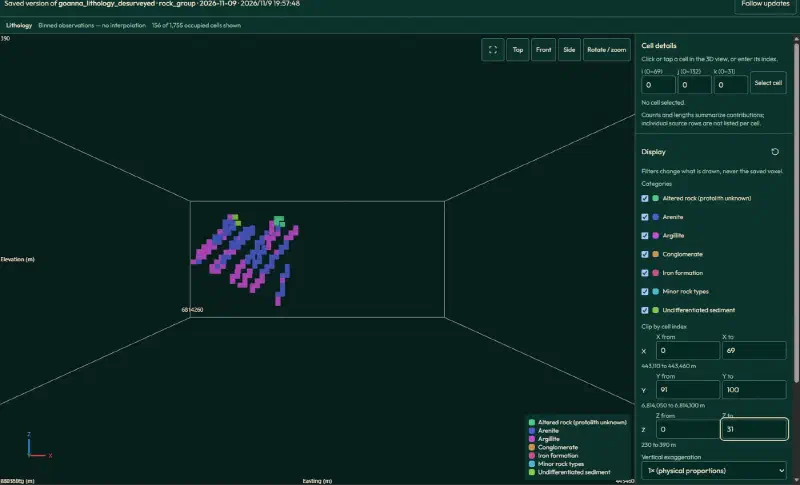
For an east-west slice, set Y from 91 to 100 (northing 6,814,050 to 6,814,100 m), click Front and zoom in. It shows 156 cells on the same strip of ground as the cross-section.
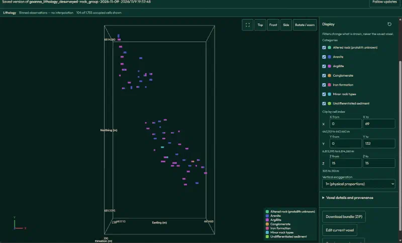
Similarly, for a level map, set Z from and Z to both to 15 (305 to 310 m elevation) and click Top. You get 104 cells.
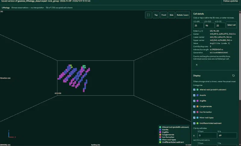
Finally, enter cell (25, 96, 22) under Cell details to check one result. It shows Argillite from five rows over 6.07 m. GDDH0060 is the only hole in this cell, and by hand the five rows give:
| Interval (m) | Rock | Length in cell (m) |
|---|---|---|
| 100.1–102.4 | Argillite | 2.19 |
| 102.5–103.15 | Argillite | 0.65 |
| 105.7–106.5 | Argillite | 0.78 |
| 103.15–103.9 | Arenite | 0.75 |
| 104.0–105.7 | Arenite | 1.70 |
Argillite totals 3.62 m and Arenite 2.45 m, so Argillite labels the cell. Together they make the 6.07 m in the panel. However, this cell hides 2.45 m of Arenite that the strip log still shows.
Limits of This Lithology Visualisation
These views visualise lithology from drillhole logs as recorded, so they also carry the limits of those records:
- Not a geological interpretation. Nothing is drawn between holes, so these views cannot show how rock units connect.
- One label per cell. A 5 m cell keeps the rock with the longest total length. Thin units can vanish, and ties go to the label that sorts first.
- Grouped labels. The 3D table merges rare codes into
Minor rock types, while the strip log keeps the original names. - Projected hole ends. Past the last kept survey station, holes continue in a straight line. That reaches 53.77 m in GDDH0100, so treat deep ends with care.
- Colours differ between views. The strip log and section use fixed colours. The 3D viewer assigns its own from the label text, so read each legend.
- Below-detection results. The strip log marks them separately, while the composites count them as 0 g/t. Assay detection limits vary by lab, so state your choice.
- Perspective. The 3D views use perspective, so do not measure distances on them.
- Check the written summary. Treat the saved tables and figures as the result, and verify historical drilling data against its source. We recomputed every count, depth and composite in this guide from the raw files.
FAQs
What is a lithology log in a drillhole?
A lithology log records the rock type along a drillhole, interval by interval, usually as a from depth, a to depth and a rock code. Geologists write it while examining core or chips. Because codes vary between companies, a log normally comes with a dictionary that explains what each code means.
How is a strip log different from a cross-section?
A strip log draws one hole as a vertical column, with rock type, weathering, structures and assays side by side against depth. A cross-section places several holes on one slice of ground at their true positions and angles. Use the strip log for detail and the section for comparing holes.
Why leave out some downhole survey readings?
Magnetic survey tools read the Earth’s magnetic field, so magnetic rock can push their azimuth off course. In hole GDDH0057, one magnetic reading differs from the gyroscope readings around it by about 70 degrees. Where a hole has gyroscope or aligner readings, using only those avoids false bends in its path.
What happens to intervals with no rock record?
Precollar and core-loss intervals have no observed rock, so they get the label No data. The 3D builder counts them as left out, which keeps them from becoming a rock class. In this guide, 1,049 of 5,695 intervals are treated this way, and the 2D figures draw them in light grey.
Does a lithology voxel model predict rock between holes?
No, an observation voxel model fills only the 3D cells that drillholes physically cross and leaves the rest empty. Here, just 1,755 of 297,920 cells hold a rock type. Predicting rock units between holes needs geological interpretation or interpolation, which is a separate step after checking the measured data.
Can I use my own drillhole logs instead of WAMEX files?
Yes, any logs work if they have hole IDs, collar positions, downhole surveys and from and to depths with rock codes. Change the first prompt to match your column names, or skip it if your tables are already clean. Keep a code dictionary, and check the agent’s tables against your source files.
Visualise Lithology in Geocluster
Open the Geocluster web workspace to visualise lithology from drillhole logs in your browser, without writing code or setting up servers. Next, create a project, upload the five WAMEX files (or your own logs), and send the four prompts above to draw a strip log and a cross-section. Then run the voxel wizard to build the 3D model.