TL;DR: Elastic Weight Consolidation (EWC) slows down catastrophic forgetting during sequential training by anchoring each parameter \(\theta_i\) to its prior task optimum \(\theta^*_{A,i}\) with a quadratic penalty weighted by diagonal Fisher Information \(F_i\). While virtual Fisher springs work cleanly on compact vision and RL networks (extended via Online EWC and Kronecker curvature), billion-parameter Transformers hit steep memory overhead, drifting local Taylor approximations, and polysemantic neurons. Modern LLM pipelines therefore replace or pair full-parameter EWC with Low-Rank Adaptation (LoRA), bounded replay buffers, or exact output-space KL divergence against a frozen base checkpoint.
Why Sequential Fine-Tuning Overwrites Old Skills
Suppose you train a neural network or an agent inside a recursive self-improvement loop on Task A (such as classifying medical images or answering SQL queries) until it reaches strong accuracy at parameter vector \(\theta^*_A\). Next week, new data arrives for Task B, and you continue running gradient descent starting from \(\theta^*_A\).
Standard gradient descent only sees the loss surface of Task B. Because deep networks are heavily overparameterised, many different weight configurations achieve low loss on Task B, yet only a small subset of those configurations also preserves low loss on Task A. Left unconstrained, the optimiser takes the steepest path downhill on Task B, marches straight out of Task A’s low-loss valley, and wipes out earlier competence within a few hundred steps.
In their foundational paper on Elastic Weight Consolidation, Kirkpatrick et al. (2017) proposed a clean geometric solution: find a parameter region where both Task A and Task B achieve low error by allowing Task B to move weights freely along directions that barely mattered to Task A, while stiffly resisting movement along directions that were critical to Task A.
How Elastic Weight Consolidation Works
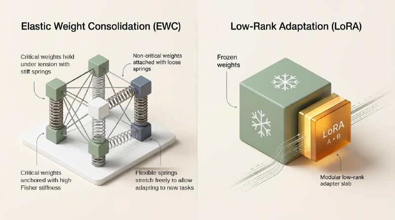
The phrase elastic weights comes directly from the physics of a mechanical spring. Imagine anchoring every weight \(\theta_i\) to its Task A value \(\theta^*_{A,i}\) with an individual spring:
- If changing \(\theta_i\) ruins Task A’s predictions, attach a stiff spring so Task B can barely budge it.
- If Task A’s output stays almost unchanged when \(\theta_i\) wiggles, attach a loose spring so Task B can repurpose that capacity.
From Bayesian Posteriors to Virtual Springs
Mathematically, EWC derives this spring from Bayes’ rule. Given two independent datasets \(\mathcal{D}_A\) and \(\mathcal{D}_B\), the log-posterior over parameters \(\theta\) after seeing both tasks decomposes as:
$$\log p(\theta \mid \mathcal{D}_A, \mathcal{D}_B) = \log p(\mathcal{D}_B \mid \theta) + \log p(\theta \mid \mathcal{D}_A)-\log p(\mathcal{D}_B)$$The first term \(\log p(\mathcal{D}_B \mid \theta)\) is just the negative Task B training loss \(-\mathcal{L}_B(\theta)\). All information learned from Task A lives inside the prior term \(\log p(\theta \mid \mathcal{D}_A)\), which is intractable to compute exactly once \(\mathcal{D}_A\) is no longer replayed.
EWC approximates \(\log p(\theta \mid \mathcal{D}_A)\) using a Laplace approximation: a second-order Taylor expansion around the Task A optimum \(\theta^*_A\) (where the first derivative vanishes), keeping only the diagonal entries of curvature. Dropping constants yields the EWC training objective:
$$\mathcal{L}_{\text{EWC}}(\theta) = \mathcal{L}_B(\theta) + \frac{\lambda}{2} \sum_i F_i (\theta_i-\theta^*_{A,i})^2$$Here, \(\lambda > 0\) controls the overall trade-off between preserving Task A and fitting Task B, and \(F_i\) is the \(i\)-th diagonal entry of the Fisher Information Matrix evaluated at \(\theta^*_A\):
$$F_i = \mathbb{E}_{x \sim \mathcal{D}_A,\, y \sim p_\theta(\cdot \mid x)} \!\left[ \left( \frac{\partial \log p_\theta(y \mid x)}{\partial \theta_i} \right)^2 \right]_{\theta = \theta^*_A}$$Take the gradient of that penalty with respect to \(\theta_i\), and you get Hooke’s Law (\(F_{\text{spring}} = k \cdot \Delta x\)) with spring constant \(k_i = \lambda F_i\):
$$\frac{\partial}{\partial \theta_i} \!\left[ \frac{\lambda}{2} F_i (\theta_i-\theta^*_{A,i})^2 \right] = \lambda F_i (\theta_i-\theta^*_{A,i})$$Why use squared log-likelihood gradients for \(F_i\)? By a classic statistical identity, the expected outer product of log-likelihood gradients equals the negative expected Hessian (the local curvature of the loss valley) at the optimum. Computing exact second derivatives across millions of weights is expensive, whereas squaring first-order gradients from a single pass over a sample of Task A inputs takes ordinary backpropagation.
Online EWC and Kronecker Curvature Across Many Tasks
Two limitations showed up quickly as researchers moved beyond two-task benchmarks:
- Linear memory growth across tasks: In naive multi-task EWC, learning \(T\) sequential tasks requires storing \(T\) separate anchor checkpoints \(\theta^*_t\) and \(T\) Fisher tensors \(F^{(t)}\). In Progress & Compress, Schwarz et al. (2018) resolved this with Online EWC, maintaining a single running Fisher accumulator \(\tilde{F}^{(t)} = \gamma \tilde{F}^{(t-1)} + F^{(t)}\) (with decay factor \(\gamma \le 1\)) anchored at the latest consolidated parameter vector \(\theta^*_{t-1}\).
- Ignoring cross-parameter interactions: Diagonal EWC treats every weight coordinate independently, zeroing out off-diagonal couplings between weights in the same layer. Ritter, Botev, & Barber (2018) introduced structured Laplace approximations, using Kronecker-factored Approximate Curvature (K-FAC) to capture layer-wise parameter correlations without storing a full \(|\theta| \times |\theta|\) matrix.
Why Classic EWC Hits Friction at LLM Scale
On compact MLPs, ConvNets, and Atari Q-networks, EWC and Online EWC provide a clean baseline when replay data cannot be stored. When you scale up to a 7B or 70B Transformer, however, four practical bottlenecks appear:
| Bottleneck | What Happens in Classic Full-Parameter EWC | Modern LLM Workaround |
|---|---|---|
| VRAM footprint | Requires keeping FP32/BF16 copies of \(\theta^*_A\) and diagonal Fisher \(F_i\) alongside model weights, gradients, and Adam states (\(+2\times\) parameter memory) | Freeze base weights (often in 4-bit) and restrict trainable parameters via LoRA or gradient masking (Tan et al., 2026) |
| Polysemantic weights | A single Transformer weight participates in many unrelated features at once, blurring per-weight importance scores (Ning et al., 2026) | Regularise sparse latent features, activations, or output token distributions directly |
| Local curvature decay | Fisher \(F_i\) only describes local quadratic curvature right at \(\theta^*_A\); after large updates, the Taylor approximation drifts | Use periodic experience replay or exact KL divergence against the frozen base policy |
| Coordinate symmetries | Re-scaling SwiGLU/attention projections or low-rank factors \((B R^{-1})(R A)\) changes coordinates without changing model outputs | Apply subspace orthogonality, adapter resets, or function-space regularisation |
Recent empirical work highlights these exact trade-offs:
- Polysemanticity blurs weight springs: Using SAE-guided activation regularisation, Ning et al. (2026) show why per-weight EWC often underperforms on LLMs: because individual MLP and attention weights are polysemantic (superposing many distinct concepts), stiffening a weight to protect one capability inadvertently blocks plasticity for unrelated downstream skills, or vice versa.
- Masking instead of quadratic storage: With Fisher-guided gradient masking, Tan et al. (2026) use diagonal Fisher scores to generate adaptive binary gradient masks during LLM updates, avoiding the memory overhead of storing full historical reference checkpoints.
EWC vs. LoRA in Continual Learning
When engineers fine-tune open-weight LLMs today, the most common starting point is Low-Rank Adaptation (LoRA), which freezes the pre-trained weight matrix \(W_0 \in \mathbb{R}^{d_{\text{out}} \times d_{\text{in}}}\) and learns a low-rank update \(\Delta W = \frac{\alpha}{r} B A\) with \(r \ll \min(d_{\text{in}}, d_{\text{out}})\).
How does LoRA relate to EWC?
- Implicit subspace regularisation: Analysing how LoRA forgets less, Biderman et al. (2024) demonstrate on code and math continual adaptation that restricting gradient updates to a low-rank subspace acts as a strong structural regulariser: LoRA preserves out-of-domain base capabilities far better than unconstrained full fine-tuning, even with zero Fisher penalties.
- Combining weight regularisation with low-rank adapters: LoRA alone does not eliminate forgetting when multiple adapters or sequential tasks overwrite the same subspace. Studying low-rank weight regularisation, Zheng et al. (2026) analyse how classic weight regularisation interacts with parameter-efficient continual learning (PECL), showing how curvature penalties can be adapted specifically to low-rank parameterisations where naive per-coordinate penalties suffer from factorisation ambiguities.
- Zero-copy functional anchoring: Remember that EWC’s quadratic penalty \(\frac{1}{2}(\theta-\theta^*)^\top F (\theta-\theta^*)\) is mathematically a second-order Taylor approximation to the Kullback-Leibler divergence \(D_{\text{KL}}(p_{\theta^*} \parallel p_\theta)\). With LoRA, the untouched base weights \(W_0\) remain sitting in GPU memory; toggling the adapter off during a forward pass (
with model.disable_adapter():) lets you apply exact anchored KL fine-tuning against the base model without storing a second reference checkpoint or approximating curvature with a diagonal matrix.
In short: choose EWC / Online EWC when updating compact dense models sequentially under strict zero-replay rules; choose LoRA + bounded replay or functional KL anchoring (or hybrid low-rank Fisher methods) when adapting billion-parameter Transformers.
Implementing and Benchmarking EWC in PyTorch
The fastest way to build intuition for elastic weights is to inspect a minimal implementation and then benchmark it against replay and adapter baselines using established open-source libraries.
Minimal 25-Line PyTorch EWC Module
Below is a self-contained PyTorch implementation of diagonal EWC that works on any nn.Module classifier or language head:
import torch
import torch.nn as nn
import torch.nn.functional as F

class DiagonalEWC:
    def __init__(self, model: nn.Module, dataloader, device: str = "cuda"):
        self.params = {
            n: p.detach().clone()
            for n, p in model.named_parameters()
            if p.requires_grad
        }
        self.fisher = {n: torch.zeros_like(p) for n, p in self.params.items()}
        self._estimate_fisher(model, dataloader, device)

    def _estimate_fisher(self, model: nn.Module, dataloader, device: str):
        model.eval()
        n_samples = 0
        for x, y in dataloader:
            x, y = x.to(device), y.to(device)
            model.zero_grad()
            log_probs = F.log_softmax(model(x), dim=-1)
            # Empirical Fisher on ground-truth or sampled labels
            loss = F.nll_loss(log_probs, y, reduction="sum")
            loss.backward()
            for n, p in model.named_parameters():
                if p.requires_grad and p.grad is not None:
                    self.fisher[n] += p.grad.detach().pow(2)
            n_samples += x.size(0)
        for n in self.fisher:
            self.fisher[n] /= max(1, n_samples)

    def penalty(self, model: nn.Module) -> torch.Tensor:
        loss = torch.tensor(0.0, device=next(model.parameters()).device)
        for n, p in model.named_parameters():
            if n in self.fisher:
                loss = loss + (self.fisher[n] * (p - self.params[n]).pow(2)).sum()
        return 0.5 * loss
During Task B training, you simply add ewc_lambda * ewc.penalty(model) to your task loss before calling .backward().
Open-Source GitHub Repositories to Benchmark EWC
Rather than maintaining custom boilerplate for multi-task streams and metrics, you can experiment directly with these active, independent open-source repositories:
- ContinualAI Avalanche library: The standard end-to-end PyTorch toolkit (
ContinualAI/avalanche) for continual learning. It ships with both classic per-task EWC (mode="separate") and Schwarz et al.’s Online EWC (mode="online"), making it straightforward to benchmark EWC head-to-head against Experience Replay (ReplayPlugin) and Learning without Forgetting (LwFPlugin):
pip install avalanche-libfrom avalanche.training.supervised import EWC
strategy = EWC(
model=my_model,
optimizer=my_optimizer,
criterion=my_criterion,
ewc_lambda=400.0,
mode="online",
decay_factor=0.9,
train_mb_size=64,
train_epochs=3,
)- PyTorch continual-learning suite: Gido van de Ven’s readable repository (
GMvandeVen/continual-learning) comparing EWC, Online EWC, Synaptic Intelligence (SI), LwF, and experience replay across Task-IL, Domain-IL, and Class-IL protocols, highlighting where parameter regularisation succeeds (Task/Domain-IL) versus where replay is required (Class-IL). - Minimal EWC notebook: A concise standalone PyTorch implementation (
moskomule/ewc.pytorch) illustrating Permuted MNIST accuracy with and without diagonal Fisher springs. - Hugging Face PEFT: For LLM workloads (
huggingface/peft), attach rank-constrained LoRA adapters (LoraConfig) to frozen 4-bit or BF16 Transformers and callwith model.disable_adapter():whenever you want to replace diagonal weight springs with exact output-space KL anchoring.
FAQs
What is Elastic Weight Consolidation (EWC) in continual learning?
Elastic Weight Consolidation is a regularisation method that slows catastrophic forgetting by adding a quadratic penalty around parameters learned on earlier tasks. Each weight’s penalty stiffness scales with its diagonal Fisher Information score, keeping critical weights near prior optima while letting less sensitive weights adapt freely.
Why does classic EWC struggle on large language models?
Full-parameter EWC requires storing reference weights and Fisher tensors alongside optimiser states, roughly tripling parameter memory on billion-parameter Transformers. In addition, Transformer weights are polysemantic (encoding multiple unrelated features in the same coordinates), and local quadratic Taylor approximations lose accuracy once fine-tuning moves far from the anchor.
How is Online EWC different from standard EWC?
Standard multi-task EWC stores a separate reference checkpoint and Fisher tensor for every completed task, causing memory and penalty cost to grow linearly with task count. Online EWC compresses prior tasks into a single decaying running Fisher average anchored at the most recent consolidated checkpoint.
Should you use EWC or LoRA when fine-tuning LLMs sequentially?
For open-weight LLMs, starting with Low-Rank Adaptation (LoRA) on a frozen base model is usually more practical than full-parameter EWC. LoRA restricts updates to a small subspace, cuts VRAM overhead, and lets you compute exact output-space KL divergence against the frozen base via disable_adapter().
Can EWC completely prevent catastrophic forgetting without replay data?
No. Diagonal EWC slows forgetting effectively in task-incremental and domain-incremental settings, yet typically degrades in class-incremental streams or under large distribution shifts where off-diagonal weight interactions matter. Combining parameter-efficient adapters with a small rehearsal or sliding-window buffer provides much stronger retention in practice.