TL;DR: In an online SFT loop, the policy at step \(t+1\) is trained on the filtered trajectories produced at step \(t\), turning every output into a candidate training row and creating a training-level explore-exploit tradeoff that a frozen policy never faces. A trajectory’s value splits into its immediate return plus a discounted improvement in the next policy’s future value, allowing selection over multiple update cycles to preserve low-return instrumental strategies (such as a fast first attempt that triggers an informative error message) without any curiosity bonus or exploration reward in the loss. Under RLVR the same tension appears as entropy collapse and a pass@1 gain that the base model undoes at large \(k\), which is why RLVR carries the exploration term explicitly through entropy controls and pass@k objectives while online selection loops carry it through the environment filter and update cadence.
Why a Frozen Policy Has No Explore-Exploit Tradeoff
Take a coding agent whose weights never change after deployment, \({\theta }_{t}={\theta }_{0}\) for every \(t\). Each action it takes changes the environment state, \({E}_{t+1}=T({E}_{t},{a}_{t})\), and nothing else. Its only lever on performance is the immediate outcome of each trajectory, written \(\Delta R({\tau }_{t})\): the disk space freed, the test passed, the balance moved. The classic explore-exploit tradeoff exists only inside an episode, with no recursive self-improvement carrying what was learned into the next.
Now let the loop update the weights. After a bounded window of episodes, the trajectories that met a selection criterion \(S(\tau )=1\) are collected into a buffer \({B}_{t}\), and the policy is retrained on it: \({\theta }_{t+1}=U({\theta }_{t},{B}_{t})\). In Eigenform’s loops the update trains a fresh LoRA adapter with a modified SFT loss on that window, two components chosen separately. Whatever the update rule, the consequence is the same: every trajectory the agent produces is now a candidate training example for its own successor, and the agent’s outputs shape the policy that will face the next environment, the dependence behind self-induced distribution shift.
Direct vs. Instrumental Strategies: Decomposing a Trajectory’s Value
The two terms
Write \(V(\theta ,E)\) for the expected cumulative return of policy \(\theta\) in environment \(E\) over some horizon. In the frozen regime the value of a trajectory is \(\Delta R({\tau }_{t})\) and nothing more. In the online regime it gains a second term, scaled by a discount \(\beta\) that reflects how far ahead the loop effectively looks:
$$\text{Value}(\tau_t) = \Delta R(\tau_t) + \beta \, \mathbb{E}_{E_{t+1}}\big[V(\theta_{t+1}, E_{t+1})-V(\theta_t, E_{t+1})\big]$$The bracket is the improvement in future performance that comes from training on \({\tau }_{t}\), conditional on \(S({\tau }_{t})=1\). If the trajectory is filtered out, the bracket is zero and the trajectory was worth exactly its immediate return. If it is kept, the bracket can be large even when \(\Delta R({\tau }_{t})\) is small, because what it teaches the next policy matters more than what it achieved.
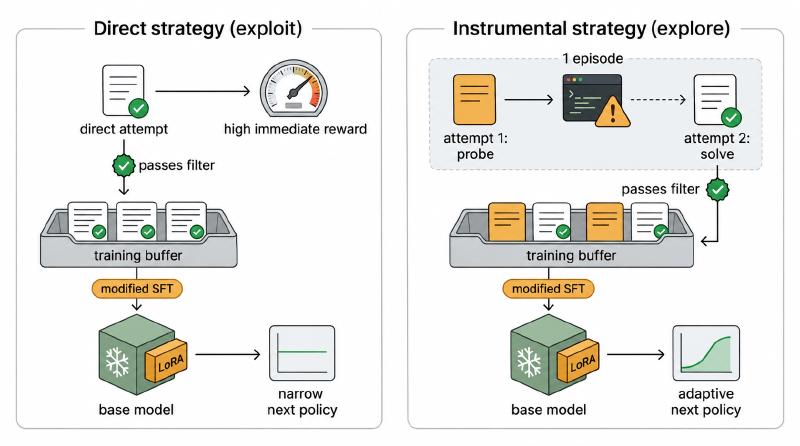
That split defines the two strategy types the table compares. A direct strategy produces \(\Delta R>0\) now: run the known-good cleanup command, submit the memorised solution. An instrumental strategy produces low immediate return but high information gain \(\mathcal{I}(y, E_t)\), and it is worth keeping when the environments that follow pay more to a policy that has seen that information:
$$\mathbb{E}_{E_{t'} \mid \mathcal{I}(y, E_t)}\big[\Delta R(y', E_{t'})\big] > \mathbb{E}_{E_{t'}}\big[\Delta R(y', E_{t'})\big]$$| Direct strategy | Instrumental strategy | |
|---|---|---|
| Immediate return \(\Delta R\) | Positive | Near zero |
| Information gain \(\mathcal{I}(y, E_t)\) | Low: confirms what the policy already does | High: error messages, probes, variants that fail informatively |
| What it adds to \({B}_{t}\) | Rows that repeat the current best approach | Rows that make the next window’s successes possible |
| How it reads in metrics | High pass@1 | Lower pass@1, higher success after several attempts |
What our agents did
In our paper Survival is the Only Reward we attempted to measure these phenomena explicitly. Coding agents were retrained for thirteen versions on their own successful episodes in an environment where a failed compile cost nothing but a retry. In one lineage, online pass@1 fell from 55 percent at the third version to zero from the sixth onward, while the share of its code blocks that compiled and ran rose from 21 percent at the first version to 85 percent at the thirteenth. The agents had no scratchpad, no conversational memory and no instruction to explore. They converged on generating a plausible first attempt quickly, reading the error, and iterating, and that pattern was written into the weights one version at a time because the episodes it produced kept passing the filter.
Exploration Without Reward: How Selection Pays for the Second Term
Exploration in RL is usually bought explicitly. Curiosity-driven exploration in the style of Pathak, Agrawal, Efros and Darrell (2017) adds an intrinsic reward equal to the agent’s prediction error about the next state, so visiting the unfamiliar is paid for inside the objective.
Random network distillation, from Burda, Edwards, Storkey and Klimov (2018), pays a novelty bonus from the error of predicting a fixed random network’s features. Both work, and both make exploration a term the designer has to weight against the task reward.
The online SFT loop in Survival is the only Reward has no such term. Its loss is a modified cross-entropy on kept trajectories, with no entropy bonus, no information-gain reward and no curiosity signal. The second term of the decomposition is paid for by a different mechanism: a policy that keeps producing instrumental trajectories reaches more future successes, those successes pass the filter, and the next adapter is trained on them. Over several update cycles that selection appears to resolve the explore-exploit tradeoff in favour of policies that leave the future maximally learnable, rather than policies that index fully on the present environment. That is to say, strategies that maximise informative failure while minimising overall failure are retained in preference to strategies that simply minimise overall failure. Because experience is acquired first, by the environment’s selection, and optimised afterwards without an explicit policy gradient or reward model, we describe the result as approximate policy-free online learning.
The same loop carries a known risk from the model-data feedback literature. Shumailov and colleagues (2023) showed that iterative fine-tuning on a model’s own outputs erodes the tails of the distribution it started from, and a filter that keeps only direct strategies accelerates that erosion. Instrumental trajectories are the counterweight: exactly the rows a greedy filter would discard, and exactly the rows that keep the next policy able to adapt.
RLVR Faces the Same Tradeoff, and Pays for It Explicitly
Where a reliable checker exists, reinforcement learning with verifiable rewards is the stronger default, and GRPO as used in DeepSeek-R1 is the reference implementation. The decomposition still applies: a rollout is worth its verified reward plus whatever its advantage teaches the next policy. Because the gradient is driven by the first term, the policy sharpens toward paths that already score, and the second term shrinks as it does. Three results from 2025 describe that drift, a thread that this year’s work on entropy interventions in RLVR continues.
- Cui and colleagues traced entropy collapse in RLVR to the covariance between a token’s probability and its advantage: confident, high-advantage tokens pull entropy down early, and performance plateaus with it.
- Yue and colleagues found that RLVR models beat the base model at pass@1 but lose to it at large k, a sign that training exploited paths the base model already contained rather than widening coverage.
- Chen and colleagues trained on a pass@k reward over a set of samples, which puts the learnability term back into the objective as an explicit balance between exploration and exploitation.
The difference between the two paradigms is where the exploration term lives. For RLVR it sits in the reward or the trainer, tuned through entropy controls, clipping ranges or set-level objectives. For the selection loop it sits in the environment, which saves that tuning but demands a filter tied to a conserved environmental quantity and update cycles frequent enough for the second term to matter. Neither is free, and the choice should follow what the environment can verify, a comparison this site has drawn for sparse-feedback agents.
Reading the Tradeoff in Your Own Loop
Three practical consequences follow for anyone who wants to read the explore-exploit tradeoff in an iterative fine-tuning loop over an agent’s own trajectories.
- Measure the second term, not only the first. Online pass@1 is a direct-strategy metric. A falling first-attempt rate next to a rising rate of eventual success is the signature of instrumental strategies being learned, the pattern behind first-attempt pass@1 drops. Track success over attempts, compile rate and the pass@k curve at several values of k.
- Let the filter decide on outcomes, not on the shape of the trajectory. A filter that keeps only clean one-shot solutions selects direct strategies and deletes variance; a filter on environmental effect keeps whatever path reached one. Self-training pipelines such as ReST-EM filter on verified correctness and report gains that saturate after a few iterations, consistent with a filter that admits direct strategies alone.
- Set the update cadence with the discount in mind. The second term is discounted by how soon training on a trajectory changes the policy that acts next. Infrequent updates on long windows push the discount toward zero and the loop toward a frozen policy; a bounded window and a fresh adapter per cycle, as in a nightly LoRA schedule, keep it high enough for instrumental trajectories to pay off.
FAQs
Is this the same explore-exploit tradeoff as in bandits and RL?
It is the same tension one level up. In bandits and exploration in RL, the agent trades off actions to estimate values within a fixed learning problem. In an online SFT loop the agent’s outputs also decide what its successor is trained on, so the tradeoff covers training data as well as actions, with no exploration term in the loss.
Does a deliberately imperfect first attempt count as reward hacking?
Not under the axiom these loops run on: no method that gets the reward is a bad method. The environment measures a conserved quantity, space freed or tests passed, and a trajectory that reaches it through a cheap failed probe has adapted to that environment. Whether a reported metric such as pass@1 agrees is a question about the metric.
What sets the discount in practice?
Nothing in the loss. The discount is set by the loop’s mechanics: how often the policy is updated, how long the training window is, and how much one trajectory can move a fresh adapter. Frequent updates on bounded windows raise it; a large cumulative buffer updated rarely lowers it toward the frozen-policy case where only immediate return counts.
How do online SFT loops explore without a curiosity bonus or entropy term?
Online SFT loops explore through multi-cycle environmental selection rather than an explicit term in the loss function. When an agent takes an informative probe that yields low immediate return but unlocks a subsequent solution, the whole episode passes the survival filter and enters the training buffer, reinforcing that exploratory sequence in the next adapter.
How does the explore-exploit tradeoff differ between online SFT and RLVR?
RLVR handles the explore-exploit tradeoff inside the optimizer using token-level advantages, clipping ranges, entropy bonuses, or pass@k rewards. In contrast, an online SFT selection loop leaves the loss function as modified cross-entropy and shifts exploration control to the environment filter, the retry budget within each episode, and the sliding-window update cadence.
Why does filtering only one-shot successes hurt self-training agents?
Filtering for clean one-shot solutions keeps only direct strategies that confirm what the current policy already knows. Discarding multi-step recovery traces removes the error messages and diagnostic probes that teach the next adapter how to adapt, which accelerates distribution tail erosion and causes iterative self-training gains to plateau after a few cycles.
Eigenform is a company building self-training open source models and frameworks. You can try them on GitHub.