Key Takeaways
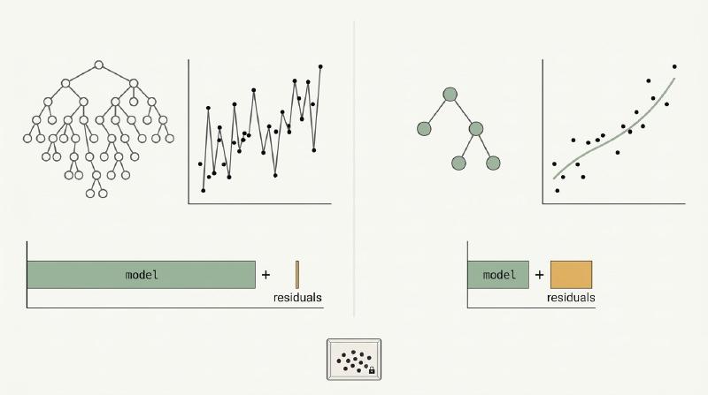
- An agent that proposes hypotheses and is scored on held-out fit alone drifts toward bloated expressions, because every extra term buys a little fit and costs nothing. That is a property of the objective, not a fault of the agent.
- The minimum description length (MDL) principle repairs the objective: score a hypothesis by the bits needed to state it plus the bits needed to encode the data given it. Fit and complexity then share one unit, so the trade-off needs no hand-tuned weight.
- Solomonoff induction is the uncomputable ideal behind MDL: weight every hypothesis by two to the power of minus its program length. A two-part code over a restricted expression grammar is the practical approximation.
- A complexity charge does not cover search multiplicity. Scoring thousands of candidates against one held-out set leaks information, so a hypothesis scorer also needs a query budget or a fresh holdout per round.
TL;DR
When an LLM (Large Language Model) agent searches a space of candidate rules and is rewarded for held-out fit alone, the winning rule is usually the one with the most free parameters. Minimum description length replaces that reward with a code length, bits for the hypothesis plus bits for the residuals it leaves, which is Occam’s razor stated as an objective. In practice that means parsing each candidate into a restricted expression tree, charging for every node and constant, subtracting the charge from the held-out gain, and bounding how often the holdout may be queried.
Why Agent-Proposed Hypotheses Overfit
Hypothesis search loops now run at scale: an LLM or an evolutionary search proposes candidate rules (equations, predicates, decision rules), a scorer evaluates each one on data, and the best candidates seed the next round. LLM-SR by Shojaee et al. (ICLR (International Conference on Learning Representations) 2025) is a representative loop, with the model writing equation skeletons as programs and a fitter estimating their constants. Overfitting prevention in this setting is harder than in a single model fit, because the proposer can enlarge the hypothesis class at will: one more term, one more conditional, one more fitted constant.
The first instinct is to treat a 40-term expression that scores well on the holdout as a failure of the agent. It is not. The scorer asked for held-out fit and the agent delivered held-out fit, so any method that secures the score is a valid solution to the problem as stated. Overfitting prevention therefore belongs in the objective, where it changes what wins, and not in a prompt that asks the proposer to be parsimonious.
Solomonoff Induction and the Minimum Description Length Principle
Ray Solomonoff’s 1964 theory of inductive inference gives every hypothesis a prior weight of \({2}^{-K(H)}\), where \(K(H)\) is the length of the shortest program that produces it, and predicts with the Bayesian mixture over all programs. The mixture’s total expected prediction error on any computable source is bounded by a constant proportional to that source’s program length, which is why the prior is called universal. Rathmanner and Hutter (2011) give the full treatment, and the catch for practitioners is that \(K(H)\) is not computable, so the ideal cannot be run.
Jorma Rissanen’s minimum description length principle (1978) keeps the shape of the argument and drops the uncomputable part. Fix a description language for hypotheses, encode the data through the hypothesis, and prefer the hypothesis under which the total code is shortest:
$$ L(D) = L(H) + L(D \mid H) $$Here \(L(H)\) is the bits needed to state the hypothesis and \(L(D \mid H) = -\log_2 P(D \mid H)\) is the bits needed to encode the data given it, which is the negative log-likelihood. Grünwald’s tutorial (2004) is the standard introduction to this two-part form and to the refined codes that improve on it.
The reason a code length prevents overfitting is arithmetic. A new parameter stated to precision \(\delta\) costs about \({\log }_{2}(1/\delta )\) bits, and it only pays for itself when it cuts the residual code by more than that. A term that fits noise lowers the residual code by a fraction of a bit per sample and cannot cover its own description, so the shortest total code leaves it out. The penalties in BIC (Bayesian Information Criterion) and AIC (Akaike Information Criterion) are coarse approximations of the same budget, with the per-parameter price fixed in advance.
Overfitting Prevention as a Code-Length Budget
Symbolic regression is where this budget has been worked out most carefully. Exhaustive Symbolic Regression (ESR), by Bartlett, Desmond and Ferreira, enumerates every expression up to a maximum complexity and ranks all of them by description length: \(L(H)\) charges each tree node by the log of the number of operator choices and each constant by the bits its precision needs, while \(L(D \mid H)\) is the residual negative log-likelihood. Desmond’s 2025 review sets out the accounting and the case for it as a single objective.
Most practical tools use a cheaper proxy. PySR, the symbolic regression library by Cranmer, charges a parsimony coefficient times the node count, keeps a Pareto front of loss against complexity, and leaves the choice of a point on that front to the user. The proxy works, but the exchange rate between fit and size is a hyperparameter, whereas a code length fixes it in bits. The table compares the three options.
| Scoring rule | What it charges | Where it falls short |
|---|---|---|
| Parameter count (AIC, BIC) | A fixed price per fitted constant | Blind to structure: a 30-node tree with two constants costs the same as a linear term |
| Weighted node count (PySR parsimony) | Operators, variables and constants, times a tunable coefficient | The coefficient has to be set per problem, and nothing ties it to the noise level |
| Two-part MDL code | Bits for the tree, bits for each constant at its useful precision, bits for the residuals | Needs a likelihood model for the residuals, and a fixed description language the search cannot extend |
A 2026 preprint shows what the charge reveals once an agent is already running. Mao and Zou audited a self-improving science agent that had admitted 252 relations through held-out prediction gates: ranked by MDL compression ratio, the top band held the canonical laws among its discoveries, and 86 percent of the ledger compressed nothing, because the prediction gate had been admitting statistical regularities. Held-out fit and compression turned out to be nearly decoupled axes, which is the strongest practical argument that overfitting prevention needs the second axis.
Putting a Complexity Charge Into a Hypothesis Scorer
The recipe has four parts: restrict the hypothesis language (parse each candidate as a Python expression, allow only names, constants, arithmetic, comparisons, conditionals and a short list of functions, and cap node count and depth); measure complexity as a weighted node count plus a per-constant charge; measure gain as the held-out log-likelihood improvement over the incumbent rule; accept only when gain minus charge is positive. The ESR repository is a reference implementation of the full code-length version, and the snippet below is the minimal form.
import ast, math

ALLOWED = (ast.Expression, ast.Name, ast.Load, ast.Constant, ast.BinOp, ast.UnaryOp,
           ast.Add, ast.Sub, ast.Mult, ast.Div, ast.Pow, ast.USub, ast.Compare,
           ast.Lt, ast.Gt, ast.IfExp, ast.Call)
EXTRA = {ast.Call: 2.0, ast.IfExp: 2.0}            # extra bits for calls and branches

def complexity_bits(src: str, const_bits: float = 8.0, max_nodes: int = 64) -> float:
    tree = ast.parse(src, mode="eval")
    nodes = list(ast.walk(tree))
    if len(nodes) > max_nodes or any(not isinstance(n, ALLOWED) for n in nodes):
        raise ValueError("outside the hypothesis language")
    bits = 0.0
    for n in nodes:
        bits += 1.0 + EXTRA.get(type(n), 0.0)
        if isinstance(n, ast.Constant) and isinstance(n.value, (int, float)):
            bits += const_bits                      # precision the data supports
    return bits

def mdl_score(src: str, nll_candidate: float, nll_incumbent: float) -> float:
    gain_bits = (nll_incumbent - nll_candidate) / math.log(2)
    return gain_bits - complexity_bits(src)         # admit when positive
When the gain is measured in bits of log-likelihood, the exchange rate is one to one and no coefficient is needed. When the gain is a ranking statistic rather than a likelihood, as in pairwise ordering accuracy, the charge has to be calibrated against a null: score random or label-permuted candidates, read off a high quantile of their gains, and set the per-bit price so that chance-level candidates fall below zero. Either way, admit on the lower confidence bound of the gain from a bootstrap over held-out samples rather than on its point estimate, since the candidate was selected for scoring well.
Why the Scorer Also Needs a Query Budget
A code length charges the hypothesis, not the search. When the proposer picks its next candidate after seeing the score of the last one, every query is adaptive, and the classical guarantee that a holdout of \(n\) samples generalises with error of order \(1/\sqrt{n}\) no longer holds for the sequence as a whole. Dwork et al. (2015) showed that answering adaptively chosen queries through a differentially private mechanism preserves validity for exponentially many of them, and their reusable holdout turns that into a rule: add noise, and answer only when the holdout disagrees with the training estimate by more than a threshold. The practical reading for a hypothesis scorer is to answer coarsely, log every query and cap the number per round.
This matters twice as much in a continual learning loop, where admitted hypotheses become training data. If the agent periodically trains a fresh adapter on the rules that passed, any leak in the scorer is written into the next generation’s prior and then amplified by a proposer that already prefers what passed last time. The same mechanism makes selecting training data by its score a way to lose generalisation, and the fix is the same: charge for complexity, bound the queries, and refresh the holdout between rounds.
FAQs
Is minimum description length just BIC with extra steps?
No. BIC charges every parameter the same price and ignores structure, so two expressions with the same parameter count cost the same. A two-part code also charges the tree, prices each constant at the precision the data supports, and keeps the residual term in the same bits, so the trade-off needs no external coefficient.
How do I set the complexity charge when my score is not a likelihood?
Calibrate against a null. Score a few hundred candidates that cannot carry signal, such as random expressions from the same grammar or real candidates scored on label-permuted data, and take a high quantile of their gains as the zero point. Then set the per-node price so that a chance-level candidate of typical size scores below zero.
Can I skip the charge by prompting the LLM to prefer simple hypotheses?
The prompt shapes proposals, but the scorer decides what survives. A proposer told to be parsimonious is still selected on the score, so across rounds the survivors drift toward whatever the score rewards, and with fit alone that means longer expressions. Put the charge in the objective and the prompt becomes a search heuristic rather than the only defence.
Does any of this change if the agent trains on the hypotheses it admits?
It raises the stakes. With a reliable checker and frequent successes, reinforcement learning with verifiable rewards is the stronger default for the training step. When the agent instead trains on filtered experience, the scorer is the filter, so its complexity charge and query budget decide the training distribution directly.
Eigenform is a company building self-training open source models and frameworks. You can try them on GitHub.