TL;DR: Classical machine learning treats the available data as an oracle, but that only holds when the data distribution is fixed. If you are interested in maintaining an inventory of currently relevant skills rather than maximising one specific policy, then trajectories from earlier policies are off-policy for the current one, and an archive weights them by volume, so the current policy becomes a shrinking share of every gradient. For an LLM agent that fine-tunes on its own trajectories, a bounded sliding window of recent rounds often matches or beats the full archive on far less data, because strategies that still pay off keep reappearing in new episodes. The practical job is to choose the retention policy deliberately, bound the age of the oldest data, and measure both forgetting and adaptation every round.
What a Replay Buffer Holds in Continual Fine-Tuning
In policy-free fine-tuning a replay buffer stores transitions so that each can be learned from more than once, in a decorrelated order. In continual learning the same structure appears as an episodic memory or rehearsal buffer: a sample of earlier tasks is interleaved with the current one so that experience replay limits catastrophic forgetting of old skills. This post is about a third use, which is where most LLM agent loops now sit. The agent acts in an environment, keeps its successful trajectories, and periodically fine-tunes on them. There is no external dataset. The buffer is the dataset.
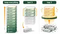
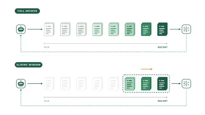
In a recursive self-improvement loop, that changes the design question: the buffer now decides which of the agent’s own past behaviours are worth imitating again. Two defaults compete, the archive (every trajectory since round one) and the sliding window (the last K rounds only), and the archive looks safe because every continual learning benchmark reports joint training on all data as the upper bound.
Why the Full Archive Is Not the Upper Bound for Self-Generated Data
Joint training is the oracle on benchmarks such as split CIFAR or permuted MNIST because every example stays valid forever: a labelled image of a cat is as correct in task ten as in task one. A trajectory produced by an agent differs in two ways. Its label is implicit (this run succeeded, under that policy, in that environment state), and its distribution is a function of the policy that produced it. Once the agent has improved, the archive is dominated by runs from weaker versions of itself, and a uniform sample from it is mostly off-policy for the model being trained. The environment moves too, since the agent’s own actions change it, which is the self-induced distribution shift that makes agent data non-stationary even when the task is fixed.
Reinforcement learning met this problem before LLM agents did. Zhang and Sutton showed at arXiv:1712.01275 that buffer size is a sensitive hyperparameter in deep Q-learning, that a buffer which is too large can hurt as well as one that is too small, and that always adding the newest transition to each update batch (combined experience replay) is a cheap remedy.
Fedus et al. then separated buffer capacity from the age of the oldest policy whose data is still in the buffer, at arXiv:2007.06700. Reducing that age improved performance at fixed capacity, while extra capacity paid off mainly in combination with n-step returns. The variable to control is staleness, and an archive lets staleness grow without bound, while a fixed window holds it constant whatever the fine-tuning objective.
How Small the Buffer Can Be
The worry about a short window is that it throws away skills the agent will need later. Two results from supervised continual learning suggest the worry is smaller than it looks. Chaudhry et al. showed at arXiv:1902.10486 that a tiny episodic memory, down to one example per class, beats methods designed specifically for continual learning, and that repeated training on that memory improved rather than hurt generalisation to past tasks, because training on later tasks acts as a data-dependent regulariser.
Ibrahim et al. found the same at LLM scale at arXiv:2403.08763: continually pre-training 405M and 10B parameter models with learning-rate re-warming, re-decaying and replay of a fraction of the earlier data matched retraining from scratch on the union of all data. What must be retained is far smaller than everything that was seen.
In an agent loop the reason is reuse. A strategy that still pays off keeps appearing in new successful episodes, because the agent keeps using it, so the window re-collects a current version of it every round. A strategy that stops appearing was tied to an environment state or a policy weakness that no longer exists, and keeping it only trains the model to repeat a behaviour that is already obsolete. Persistence comes from reuse, not from archival: the window does not need to store a skill to keep it, because the environment keeps producing fresh evidence of every skill that still matters.
Data quality beats data quantity here because the window selects for the rows that match what the model would do now. A sliding window SFT loop on this site, training a fresh LoRA adapter each round on the last few rounds of data, kept most of the archive’s gain on a fraction of its rows, which is the empirical form of the argument above.
Eigenform’s own lineages put a number on the comparison. In Survival is the Only Reward, three copies of the same Qwen 2.5 7B Instruct base were trained for thirteen versions on their own successful episodes: the Terese lineage on every row ever collected, 60,000 rows by the final version, and the Miri lineage on a three-generation window, with 500 rehearsal rows added for both. Miri kept improving on the bounded window and reached more than half of Terese’s final performance on about a quarter of the data. The paper’s reading is the one above: strategies persist through reuse, not archival, so the window re-collects every skill the environment still pays for. The approach is a serious alternative under investigation, not an established replacement for reinforcement learning.
Three Retention Policies and When Each Fits
Four retention policies for a replay buffer, and the assumption each one makes about the stream:
| Policy | What it keeps | Memory growth | Bias | Fits when |
|---|---|---|---|---|
| Full archive | Every row since round one | Linear in rounds | Towards old policies, by volume | Data is stationary and labelled externally |
| Sliding window (FIFO by round) | The last K rounds, every row | Constant | Towards the current policy | Rows are self-generated and the environment moves |
| Reservoir sampling | A uniform random sample of the whole stream, size N | Constant | None over time | A stationary external stream that must not be forgotten |
| Prioritised or selective | Rows scored by loss, novelty or reward | Constant | Towards whatever the score favours | A reliable scorer exists and its bias is wanted |
Both bounded policies fit in a few lines, with the window keyed by round rather than by row:
from collections import deque
import random

class WindowBuffer:
    """The last k rounds of trajectories, every row of each round."""
    def __init__(self, k):
        self.rounds = deque(maxlen=k)   # the oldest round leaves at k + 1

    def add_round(self, rows):
        self.rounds.append(list(rows))

    def training_set(self):
        return [row for rnd in self.rounds for row in rnd]

class ReservoirBuffer:
    """A uniform sample of size n over the whole stream (Algorithm R)."""
    def __init__(self, n):
        self.n, self.seen, self.rows = n, 0, []

    def add(self, row):
        self.seen += 1
        if len(self.rows) < self.n:
            self.rows.append(row)
        elif random.randrange(self.seen) < self.n:
            self.rows[random.randrange(self.n)] = row
Tested bounded buffers live in ContinualAI/avalanche: ReservoirSamplingBuffer(max_size=...) and ParametricBuffer(max_size=..., groupby="experience"), which splits one budget equally across every round seen so far, in avalanche.training.storage_policy. Both are updated by update(strategy) after each training experience and mixed into minibatches by ReplayPlugin.
Running Bounded Memory in an Online Fine-Tuning Loop
Run sliding window training by rounds, and train a fresh adapter per window. A fresh LoRA adapter trained from the base model on each window, rather than one adapter updated round after round, means the weights see only what the replay buffer holds, so bounding the data also bounds how far the weights drift. Training a new adapter per window, as in continual learning with nightly LoRAs, is the simplest schedule of that kind. Where a reliable verifier exists, online RL with a method such as GRPO is the stronger default, and its rollouts are a sliding window by construction, since every update uses the freshest batch.
Where feedback is sparse or arrives long after the action, a second pattern is being investigated, including at Eigenform. The agent periodically trains on the successful experiences it collected, with a modified SFT objective (the loss is changed, and the data is the agent’s own successful runs rather than curated demonstrations) on a bounded window of recent rounds, with a fresh LoRA adapter each time. The window is what keeps the training data close to the current policy without a reward model, which is why the pattern is described as approximate policy-free online learning. How it behaves over long horizons, and what it does to rare skills, are open questions rather than settled results.
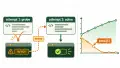
Then sweep the window and measure both ends. Run K = 1, 2, 3, 5 and the full archive, and after every round score a held-out suite of skills the base model already had (HumanEval or an instruction-following set) and a fresh suite drawn from the current environment. Log the age in rounds of the oldest row in each update, because that is the variable the RL results point at. Too short a window shows up as round-to-round oscillation and the loss of rare skills that are live but infrequent. Too long shows up as a flat fresh-suite curve while compute per round climbs. Rolling back to the previous adapter when the held-out suite drops is a safety net, not the mechanism: the control lives in the window length and the sampling rule.
FAQs
How big should the buffer be for continual fine-tuning?
Measure it in rounds of agent data and the age of the oldest row, not in bytes. Start with a window of a few rounds, sweep up to the full archive, and watch two curves: retention on a held-out prior-skill suite and gain on a fresh-task suite. The best window is the shortest one that keeps the retention curve flat.
Does a short window cause catastrophic forgetting?
It can, for skills that are still useful but rarely exercised, because the window only re-collects what the agent keeps doing. The fix is a small reservoir of older successful rows kept alongside the window, or a held-out suite that triggers a longer window when retention drops. Skills the agent uses every round are retained by reuse.
Should I use reservoir sampling or FIFO for LLM agent trajectories?
FIFO by rounds, when the trajectories come from the model’s own earlier policies. Reservoir sampling keeps a uniform sample of every policy the agent has ever been, and most of those are obsolete. Reservoir sampling fits an external stream of tasks whose examples stay valid, where the goal is never to forget any of them.
How does a sliding window differ from a replay buffer?
A sliding window is one way to manage a replay buffer: it retains every training row from only the most recent rounds, then drops older rounds as new data arrives. A replay buffer is the broader store of examples used for training. Other policies include keeping the full history, sampling a fixed-size reservoir, or prioritising selected rows.
Can I combine a sliding window with reservoir sampling?
Yes. A training set can use a recent FIFO window for current-policy data and a small reservoir of older successful rows for rare skills that may no longer appear often. Evaluate both prior-skill retention and performance on fresh tasks, because the extra older data can help preserve skills but may also reintroduce stale behaviour.