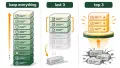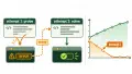
TL;DR: When fine-tuning an LLM agent across multiple generations on its own passing episodes, buffer design governs both training cost and long-horizon stability. Across 13 generations on Qwen2.5-7B-Instruct, curating the three historically highest-scoring generations (Katalin) collapsed at v12 to v13, whereas training a fresh LoRA adapter on a \(K=3\) sliding window of the three most recent generations (Miri) improved steadily without replaying older agent datasets. On a capped 15,000-row buffer (25% of full-history Terese’s 60,000 rows), the sliding window retained 58.4% of held-out MB freed per run (14,938 MB vs. 25,570 MB) and 52.6% of offline cumulative composite score (2.049 vs. 3.898, or 2.10x composite-score units per row) because useful skills keep re-entering the buffer whenever the live policy re-executes them.
Buffer Design Choices in Environment-Mediated Self-Training
In classical continual learning, a model trains sequentially on a passive external stream of tasks where dropping old examples triggers continual fine-tuning forgetting. Standard remedies fall into three mechanisms:
- Weight regularisation: Methods such as Elastic Weight Consolidation penalise updates to parameters judged important for earlier tasks.
- Experience replay: Methods such as CLEAR experience replay interleave historical trajectories alongside incoming domain examples.
- Coreset selection: Methods such as Gradient Coreset Replay retain compact subsets chosen to match historical gradient geometry.
An autonomous agent inside an active continual recursive self-improvement loop operates under different dynamics because its current policy generates candidate trajectories every round before an environment check filters them.
Following the setup formalised in the self-produced data paper, any strategy the policy still executes successfully in the current environment is regenerated automatically and re-enters recent datasets without requiring permanent archival storage.
Operational Definitions: Episode, Row, Generation, and Fresh LoRA Reset
To keep row accounting and regime comparisons exact, each object in the 13-generation container study is defined as follows:
- Episode and binary survival gate \(\mathcal{S}(\tau) \in \{0, 1\}\): In each episode of
scripts/main.py, the agent interacts with disposable Alpine Linux containers (docker/special-learn-compose) across environment discovery, cleanup strategy planning, and Python execution (with up to three retries per stage), whiledf -k /measures net disk space freed \(\Delta R(\tau)\) before and after execution:- Passing trajectory (\(\mathcal{S}(\tau)=1\), \(\Delta R(\tau) > 0\)): The agent locates seeded junk archives in
/tmp/cleanupor/var/cacheand removes them over SSH while keeping containers healthy. - Failing trajectory (\(\mathcal{S}(\tau)=0\), \(\Delta R(\tau) \le 0\)): Execution fails across retries, times out, or frees zero net bytes; the trace is archived for audit and excluded from SFT export.
- Passing trajectory (\(\mathcal{S}(\tau)=1\), \(\Delta R(\tau) > 0\)): The agent locates seeded junk archives in
- Training row: One prompt-completion pair exported from a passing episode under completion-only cross-entropy (
IGNORE_INDEX = -100on prompt tokens). Multi-stage passing episodes contribute multiple turns until a generation collects4,500agent-generated rows. - Generation (
v1tov13) and fresh-LoRA reset:v1is the untouchedQwen2.5-7B-Instructbase model, which collects Dataset1. Each subsequent checkpointv_t(v2throughv13) trains a fresh QLoRA adapter (rank=32,alpha=32, 4-bit NF4, learning rate2e-4, 3 epochs) directly from frozenv1on a selected subset of prior datasets:
Checkpoint v_{t-1} acts in sandbox -> Survival gate (Delta R > 0) keeps 4,500 agent rows (Dataset t-1)
  -> Regime rule selects prior datasets + 500 rehearsal rows per dataset
  -> Fresh QLoRA adapter trained from frozen Base Model (v1) -> Produces Checkpoint v_t
Because adapters never stack on v_{t-1}, approximation drift does not compound across rounds; continual adaptation flows through the closed-loop data channel as stronger policies write higher-yield trajectories into subsequent datasets.
How a Three-Generation Window Retains Active Skills and Prunes Stale Ones
Suppose an agent discovers strategy A (clearing /tmp caches) in v1, adds B (peer-container SSH cleanup) in v2, and adds C (log compression) in v3. As long as A and B keep freeing space during v4 and v5, the live policy keeps executing them, writing fresh A, B, and C traces into Datasets 3, 4, 5 so v6 retains them after Datasets 1 and 2 drop out. Conversely, if an environment change at v4 renders A ineffective, A stops passing \(\mathcal{S}(\tau)=1\) and ages out by v7, pruning dead habits automatically while leaving unused skills unprotected beyond \(K\) generations.
Comparing Full History, Top-3 Curation, and Sliding Window Regimes
In our Negative Space Learning paper, three lineages started from identical Qwen2.5-7B-Instruct checkpoints, shared a five-generation warm-up (v1 to v5, Datasets 1..4), and diverged from v6 through v13 under three buffer rules:
| Regime (Lineage Name) | Selection Rule for Checkpoint v_t (\(t \ge 6\)) | Datasets Used at v13 | Agent Rows at v13 | Fixed Rehearsal Rows at v13 | Total Trainer Rows at v13 | Optimiser Examples (3 Epochs, Capped at 17,000 in Annex II) |
|---|---|---|---|---|---|---|
| Full History (Terese) | All prior datasets 1..t-1 | 1..12 (12 datasets) | 54,000 | 6,000 (500 x 12) | 60,000 (100%) | Scaled with buffer (up to Annex II cap) |
| Sliding Window \(K=3\) (Miri) | Last 3 datasets {t-3, t-2, t-1} | 10, 11, 12 (3 datasets) | 13,500 | 1,500 (500 x 3) | 15,000 (25%) | Fixed 3-dataset window per round |
| Top-3 Historical (Katalin) | Top 3 prior datasets by online code-run success % | 8, 10, 11 (3 datasets) | 13,500 | 1,500 (500 x 3) | 15,000 (25%) | Fixed 3-dataset window per round |
Each generation bundles 4,500 trajectory rows collected via scripts/data_collector.py with 500 pre-cutoff Stack Exchange Paired rows (5,000 total rows per dataset), keeping the 25% ratio identical on both agent-only rows (13,500 / 54,000) and total trainer rows (15,000 / 60,000).
Raw Storage Metrics and Standardised Composite Score
Because wall-clock collection time depends on host load (dropping from 5–7 days in early generations to 10–15 hours later), each checkpoint \(i \in \{1,\dots,13\}\) tracks \(P_i\) (% of total container space freed) and \(A_i\) (mean MB freed per episode). In scripts/unweighteddeltas.py, step-over-step changes are normalised by each metric’s standard deviation across the lineage’s 13 checkpoints and summed from v1 (0.000):
Online Versus Held-Out Offline Evaluation
Every checkpoint v1 through v13 is evaluated under two protocols:
- Online metrics (Tables 2, 4, 6): Measured across the live run gathering
4,500passing rows for the next generation. - Offline held-out metrics (Tables 3, 5, 7): Measured across three independent 100-episode runs (
3 x 100episodes) seeded from held-out procedural templates (variation_1throughvariation_5), reported as mean and 95% confidence interval (n = 3runs).
Raw Storage Outcomes and Composite Scores Across 13 Generations
Experimental Scope and Statistical Boundaries
Keep three boundaries in mind before reading the endpoint numbers:
- Single lineage per regime: Terese, Miri, and Katalin were each run as one 13-generation lineage on one task and base model (
Qwen2.5-7B-Instruct); offline 95% confidence intervals measure variance across the three held-out evaluation panels, not across multiple training seeds. - Buffer row efficiency rather than collection savings: Every regime still executes the
4,500-row online collection stage each generation; the 4x reduction (15,000vs.60,000rows) applies to trainer buffer size. - Fixed window length (\(K=3\)): The published study tested \(K=3\) after a 5-generation warm-up without sweeping \(K\).
Endpoint Comparison From v1 Baseline to v13
| Regime | Held-Out Offline % Space Freed (v1 to v13) | Held-Out Offline Avg MB / Run (v1 to v13) | Online % Space Freed (v1 to v13) | Online Avg MB / Run (v1 to v13) | Offline Composite Score at v13 | Online Composite Score at v13 | Offline Composite Units per Row (Terese = 1.0x) |
|---|---|---|---|---|---|---|---|
| Full History (Terese) | 3.1% ± 1.4% to 16.6% ± 0.9% | 5,211 ± 2,275 to 25,570 ± 914 | 2.5% to 16.9% | 3,678 to 23,758 | 3.898 ± 0.927 (100%) | 3.109 (peak 3.728 at v7) | 1.00x |
| Sliding Window \(K=3\) (Miri) | 3.4% ± 1.8% to 9.0% ± 1.9% (54.2% of Terese) | 5,697 ± 2,874 to 14,938 ± 3,240 (58.4% of Terese) | 3.4% to 12.0% | 5,703 to 16,223 | 2.049 ± 1.602 (52.6% of Terese) | 3.322 | 2.10x |
| Top-3 Historical (Katalin) | 3.4% ± 1.8% to 9.0% ± 1.9%* | 7,293 ± 479 to 9,506 ± 2,165 (37.2% of Terese) | 4.5% to 4.5% (peak 13.9% at v11) | 6,549 to 6,349 (peak 20,943 at v5) | 0.482 ± 0.675 (12.4% of Terese) | -0.008 (collapsed) | 0.49x |
(Note on Table 7 of the arXiv preprint: the “% space freed” text column in Table 7 inadvertently copied Miri’s Table 5 numbers; Figure 3 and Table 7’s own MB and composite columns record Katalin rising to ~11.6% at v10 and ~10.5% at v11, then dropping to ~5.8% at v12 and ~5.7% at v13, matching its online drop from 13.9% at v11 to 4.5% at v13.)
Four Empirical Takeaways From the 13-Generation Run
- Sliding window \(K=3\) (Miri) achieves 2.10x composite score per row: Using
15,000rows instead of60,000atv13, Miri reaches58.4%of Terese’s held-out MB/run (14,938 ± 3,240vs.25,570 ± 914 MB),54.2%of held-out % space freed (9.0% ± 1.9%vs.16.6% ± 0.9%),52.6%of offline composite score (2.049 ± 1.602vs.3.898 ± 0.927), and a higher online composite endpoint (3.322vs.3.109). - Full accumulation (Terese) reaches the highest ceiling with diminishing returns: Retaining all
60,000rows delivers the highest offline storage capture (25,570 MB/run), yet Terese already reaches2.834 ± 1.868(20,089 MB/run) byv4on15,000rows before spending another45,000rows for the remaining+1.064composite units. - Top-3 historical curation (Katalin) collapses at
v12tov13: Selecting prior datasets by peak code-compile rate locks onto non-adjacent Datasets8, 10, 11, dropping online MB/run from17,114 MB(v11) to6,349 MB(v13, online composite-0.008) and offline MB/run from17,491 MBto9,506 MB(0.482composite). - General coding and cross-platform transfer hold steady: On the HumanEval coding benchmark, single-pass
pass@1 / pass@4moves slightly from77.59% / 85.37%on baseQwen2.5-7B-Instructto74.09% / 82.32%on Miriv13and75.61% / 81.71%on Teresev13, while zero-shot transfer to Windows Docker containers doubles Miri’s space freed (8.19%vs.3.63%base).
Strategy Pruning, Diagnostic Probing, and Endogenous Replay
Section 7 of the study separates directly measured diagnostics from candidate causal explanations:
- Observed strategy-variance pruning (\(D_t\)): Projecting strategy embeddings \(\phi(y)\) into PCA space with centroid \(\mu_t\) shows variance \(D_t = \mathbb{E}[\|\phi(y)-\mu_t\|^2]\) contracting from
v1tov13, consistent with Negative Space Learning concentrating mass into repeatable strategy basins rather than expanding diversity indefinitely. - Observed diagnostic error probing: Overall compile-and-run rates climb from
20.9%–33.2%atv1to57.9%–85.5%atv13while first-attemptpass@1drops to0.00%online for Terese and Katalin (0.36%for Miri), reflecting emergent probe scripts that harvest container error messages on early turns. - Candidate endogenous replay mechanism: Unlike synthetic data generators analysed in generative replay continual studies, Miri relies on live container interaction to re-execute valid strategies into
{t-3, t-2, t-1}without an auxiliary generator model. - Candidate modal fragmentation in Katalin: Fitting a fresh LoRA simultaneously on disconnected historical peaks (
8, 10, 11) likely pulls weights toward incompatible strategy modes, though multi-seed dataset-swap ablations are still needed to isolate fragmentation from single-run noise.
In contrast to passive task streams catalogued in continual learning taxonomy surveys, a recency window protects only capabilities that the active environment continues to exercise.
Running a Sliding Window Size Sweep in Code
You can inspect the original 3-stage Alpine sandbox (scripts/main.py, scripts/data_collector.py, scripts/unweighteddeltas.py) in the public Negative Space Learning repository. In our automated multi-generation training loop (scripts/run_train_loop.py), 0-indexed generations (generation_0 through generation_12) slice the trailing window_size completed folders right before launching each fresh QLoRA run:
def _collect_training_window_paths(
    generation_root: Path,
    end_generation_id: int,
    window_size: int,
) -> list[Path]:
    if window_size < 1:
        raise ValueError("training window size must be positive")

    start_generation_id = max(0, end_generation_id - window_size + 1)
    training_paths: list[Path] = []
    for generation_id in range(start_generation_id, end_generation_id + 1):
        generation_dir = generation_root / f"generation_{generation_id}"
        training_paths.append(resolve_latest_sft_training_rows_path(generation_dir))
    return training_paths
Sweeping Window Length \(K \in \{1, 3, 5\}\) Across Seeds
To test whether \(K=1\) underfits or \(K=5\) closes the remaining gap to full accumulation, hold target_training_rows = 4500, rehearsal_rows_per_epoch = 500, lora_rank = 32, and num_generations = 13 constant in your run config while varying training_window_size across {1, 3, 5, 12} and running at least three independent training.seed values per setting. Keep prior generation adapters on disk as a rollback safety net if held-out evaluation panels regress.
FAQs
Do the 15,000 vs. 60,000 row counts in sliding window SFT include rehearsal data?
Yes, each generation’s 5,000-row dataset pairs 4,500 passing agent trajectory rows with 500 pre-cutoff Stack Exchange rehearsal rows. At generation v13, a \(K=3\) sliding window trains on 13,500 agent rows plus 1,500 rehearsal rows (15,000 total), versus 54,000 agent rows plus 6,000 rehearsal rows (60,000 total) under full accumulation, preserving the exact 25% ratio.
What does 52.6% of full-history offline gains measure?
It is the ratio of standardised cumulative composite scores at v13 (2.049 for Miri’s \(K=3\) window divided by 3.898 for Terese’s full history), combining normalised step changes in % disk space freed and MB freed per run. On raw held-out metrics, Miri retains 58.4% of MB freed (14,938 vs. 25,570 MB) and 54.2% of % space freed.
Why is resetting to a fresh LoRA adapter each generation still continual learning?
Sequential updates on a single adapter compound approximation drift across rounds. Resetting each generation to a fresh LoRA on frozen v1 moves continual adaptation into the closed-loop data channel: checkpoint v_{t-1} executes stronger strategies in the sandbox, writing higher-yield passing trajectories into the buffer that trains v_t.
Does sliding window SFT prevent catastrophic forgetting across unrelated tasks?
No, a recency window only preserves task skills that the current policy keeps executing inside the active environment, while the 10% pre-cutoff rehearsal slice anchors general language and coding syntax. If a specialised task disappears from the environment for more than \(K\) generations, its trajectories age out of the window.
How should you choose the sliding window size K for an agent?
Match \(K\) to how quickly your environment shifts and how many rows each generation collects. Smaller windows (\(K=2\) or \(K=3\)) shed obsolete strategies rapidly and cap training cost in shifting environments, whereas wider windows (\(K=5\) or higher) retain rarer task variations when episodes per generation are small.