TL;DR: Best-of-N curation collapses in continual self-training when an agent’s own successes alter the environment it acts in, turning historical peak trajectories into obsolete fossils. Across 13 generations on Qwen 2.5 7B Instruct, retaining the top three historical generations (Katalin) peaked at 20,942 MB freed per run at v5 before falling back to 6,349 MB at v13, while accumulating all 65,000 past rows (Terese) plateaued after v7. Training a fresh LoRA adapter on a sliding window buffer of the last three generations (Miri, roughly 15,000 rows) sustained gains up to 16,223 MB per run and a 3.322 online composite score because strategies survive in the buffer only while the live policy keeps regenerating them.
Why Best-of-N Sampling Collapses in Non-Stationary Environments
Why does best-of-N sampling cause catastrophic collapse inside a recursive self-improvement loop operating in a non-stationary environment?
That’s the core question. Not whether collapse happens; our experiments show it clearly. Explaining why it happens changes how you curate post-training buffers.
Here’s the setup. You’re running a self-training loop. Each round, your agent generates behaviours, you pick the best ones, and you train the next version on that curated set. Best-of-N is standard practice. Rank your rollouts, keep the winners, discard the rest. It feels obviously correct: why would you train on anything less than the best?
And then the environment shifts, and your model dies in a single transition.
This isn’t hypothetical. In our Negative Space Learning experiments, three model lineages were run from the same Qwen 2.5 7B base, in the same procedurally generated Linux container environments, with the same environment-mediated selection rule (did the executed code expand the disk space it controlled or not). The only difference was how they retained data across generations:
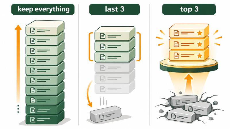
- Terese kept everything. All accumulated data from every run. By v13 she had 65,000 rows. She plateaued.
- Miri kept a sliding window of the last 3 generations. She achieved sustained, monotonic improvement: roughly 50% of Terese’s offline peak performance with 4× less data, and no catastrophic forgetting.
- Katalin kept the top 3 performing generations. The best-of-N approach. She collapsed.
Katalin is the surprising one. She did exactly what the textbooks recommend: curate aggressively, train on gold, throw away the dirt. And she didn’t just plateau; she collapsed. Performance didn’t flatten; it cratered.
The rest of this post traces why that happens. It’s not that best-of-N is a bad idea in principle. It’s that best-of-N works in a stationary environment, whereas in a non-stationary one it becomes fatal, and the non-stationarity isn’t a bug in the benchmark. It’s a direct consequence of the agent acting in its world.
Three Curation Assumptions That Break in Non-Stationary Loops
The collapse of best-of-N filtering violates three assumptions that stay hidden on static benchmarks and surface immediately during continuous online fine-tuning and test-time adaptation in non-stationary environments.
Assumption 1: Highest-Reward Filtering Always Improves Policies
Filtering for highest-reward trajectories works in stationary worlds, yet here “best” is defined against a state that no longer exists. Katalin’s top-performing runs became obsolete precisely because they succeeded. A strategy that cleared logs efficiently in generation 3 became useless in generation 6, because the logs were already gone. The agent had changed the environment, and the curated dataset was a fossil record of a past state. Katalin was hyper-selected for a niche that disappeared the moment she mastered it.
Assumption 2: The Task Distribution Stays Static During Training
In standard continual learning setups, we usually assume the task distribution shifts slowly or independently of the policy. In an interactive container environment, the agent is not just learning from the environment; it’s changing it. Every successful strategy creates a new downstream reality. Learning to clear the cache at 1pm means there will be no cache to clear at 1:05pm. The distribution isn’t drifting passively; it’s being actively rewritten by the learner. A strategy that was optimal when logs dominated the disk fails when cached images take over, and the transition can happen in a single generation.
Assumption 3: Trajectory Diversity Matters Less Than Peak Quality
Conventional wisdom says to curate aggressively: keep the gold, throw away the dirt. Yet the mediocre, diverse attempts that Katalin discarded are what allow a system to pivot when environmental conditions change. Miri survives by keeping a bridge to the next state. The sliding window doesn’t just limit memory; it preserves suboptimal variants that become useful when the environment shifts. When cache-clearing stops working, you need the half-baked compression strategies tried three generations ago. Katalin threw those away. Miri kept them around long enough for them to become relevant again.
Experiment Setup: Sliding Window SFT vs. Best-of-N Curation
Three lineages, one base model, one environment, three data retention policies. That’s the experiment.
All three started from the same Qwen 2.5 7B Instruct checkpoint. All three were dropped into the same Linux container environments: networked systems with realistic filesystem structures, permissions, processes, and failure modes. All three used the same selection rule: a behaviour survives into the training set only if executing it produced a net increase in available disk space. The environment provides no semantic feedback, no dense reward, no task-specific guidance. It just constrains what persists.
The task is open-ended disk management. The agent must discover how to free up storage in a container system: clearing caches, deleting logs, compressing files, networking between containers to find new space. Every successful action changes the state of the container. Clear the logs, and now there are no logs to clear. Compress the images, and now the disk profile looks different. The agent is not just learning in an environment; it is rewriting the environment as it learns. This is what makes the setting non-stationary in the specific sense defined earlier: the distribution doesn’t drift independently of the learner; it is caused to drift by the learner’s successes.
Each iteration generated approximately 4,500 rows of trajectory data, supplemented by 500 rows of rehearsal data drawn from the Stack Exchange Paired dataset (chosen because it predates the base model’s training cutoff, making it likely already known to the model). Like many rehearsal-based methods, this anchors the base model against drift, while a fresh LoRA adapter is trained on the retained data and applied directly to the frozen base: no adapter stacking, no parameter inheritance between rounds. The only thing that carries forward is the data.
The three lineages differ only in which data carries forward:
- Terese kept everything. Every row from every previous iteration, accumulated without pruning. Terese v2 trained on 5,000 rows; by v13 she had 60,000+. She was the data-scaling baseline: the answer to “what happens if you just keep stacking data?”
- Miri kept a sliding window of the last 3 generations. Miri v6 trained on data from v3, v4, and v5; Miri v7 on data from v4, v5, and v6. Earlier data was discarded regardless of how well it performed. She tested whether continual improvement is possible without unbounded data growth and without explicit regularisation against catastrophic forgetting.
- Katalin kept the top 3 performing generations, selected by success rate. Not the most recent: the best. This is best-of-N selection applied at the generation level: rank historical data by reward, keep the winners, throw away everything else. She tested whether aggressive quality-based curation outperforms naive accumulation or simple recency-based retention.
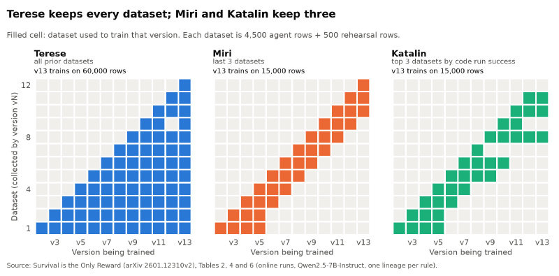
The design isolates one variable: the data retention policy. Same base model, same environment, same selection rule, same training objective (modified SFT on successful trajectories), same nightly LoRA recipe. The only difference is what survives in the buffer from one round to the next.
The comparisons we cared about were:
- Terese vs. Miri: Does a sliding window achieve competitive performance with a 4× smaller data budget? If Miri can reach even half of Terese’s peak with a fixed-size buffer, that’s evidence that the continual learning problem in non-stationary settings is not primarily a data quantity problem; it’s a data currency problem.
- Miri vs. Katalin: Does recency-based retention outperform quality-based retention? Both use a window of 3 generations. The difference is that Miri selects by time (last 3), Katalin selects by reward (top 3). If Katalin wins, quality curation works. If Miri wins, the “gold data” intuition fails in non-stationary settings, and the failure mode should be informative.
- Katalin’s trajectory specifically: Does best-of-N filtering cause collapse in a non-stationary environment, and if so, how fast? Katalin is the diagnostic canary for peak-reward curation.
Thirteen-Generation Results Across Katalin, Terese and Miri
Three lineages, thirteen versions each, one retention variable. The trajectories diverge sharply after generation 5.
Katalin: Peak Performance at v5 Followed by Total Collapse
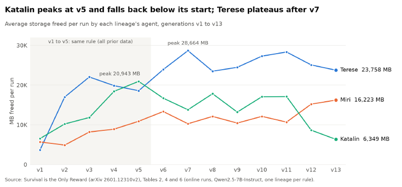
Katalin v5 was the strongest checkpoint in the early phase of the experiment. She freed 0.132% of total available space per run, higher than any Terese or Miri checkpoint at that point. Her average space freed per run reached 20,942 MB. Early on, she looked like a proof of concept for aggressive curation: train on the best, discard the rest, and get a specialist.
Then performance collapsed.
By v6, space freed dropped to 0.102%. By v7, 0.088%. The decline wasn’t gentle. By v12, she was at 0.062%; her per-step composite improvement score cratered to −2.118 in a single transition, the sharpest drop recorded by any lineage. By v13, she was back to v1 baseline levels: 0.045% space freed, 6,349 MB per run, and a −0.008 cumulative composite score. Thirteen generations of training ended right where she started.
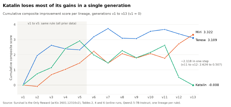
The mechanism matches what the broken assumptions predict. Katalin’s training buffer contained the top-3 performing generations. Those generations performed well against past environments: states where logs dominated the disk, where caches were full, where specific cleanup scripts worked. Once the agent cleared those logs and emptied those caches, the “best” trajectories were optimal for a world that no longer existed. Because Katalin selected by historical score rather than recency, she kept retraining on fossils.
Worse, behavioural diversity was gone. Katalin’s semantic maps show tight clusters of nearly identical, high-performing strategies. When the environment shifted and those strategies failed, there was nothing else in the buffer to fall back on. The half-baked compression attempts, mediocre networking scripts, and recovery trajectories that a wider distribution preserves had all been discarded.
Terese: Early Gains Followed by a 65,000-Row Plateau
Terese never collapsed. She simply stopped improving.
By v7, Terese was freeing 0.192% of total space per run with an average of 28,664 MB. By v13, with 65,000 rows of training data (roughly 4× what Miri ever saw at once), she was at 0.169% and 23,758 MB. The cumulative composite score oscillated without upward trend: 3.728 at v7, 3.093 at v8, 3.109 at v13. More data produced no further learning.
The bottleneck wasn’t data quantity; it was data composition. Terese’s buffer retained the entire history of every strategy she’d ever tried. Early generations discovered log-clearing; later generations discovered cache-flushing; still later ones found file compression. All of these persisted in the training set indefinitely. The model was simultaneously learning to clear logs that no longer existed, flush caches that were already empty, and compress files that had already been compressed. Later Terese versions show diffuse clusters of semantically redundant strategies (“clear cache” next to “clean out cache” next to “remove cached files”), diluting gradient signal from current states.
Terese overfit to the history of the task distribution rather than the live distribution. With complete retention and no triage mechanism, growing obsolete data steadily reduced sample efficiency.
Miri: Monotonic Gains on a Three-Generation Window
Miri v13 freed 0.120% of total space per run (16,223 MB average). On the online cumulative composite score, she reached 3.322, ahead of Terese v13’s 3.109, using a fixed-size buffer of roughly 15,000 rows against Terese’s 65,000.
On offline evaluations (three 100-iteration runs per checkpoint, 95% confidence intervals), Miri v13 achieved a mean cumulative composite score of 2.049 ± 1.602, compared to Terese v13’s 3.898 ± 0.927: roughly half of Terese’s offline score on a quarter of the data, with no catastrophic forgetting, no collapse, and no plateau within the 13-generation horizon.
The improvement held across all thirteen generations. Percentage of space freed rose from 0.034% (v1) to 0.120% (v13), a 3.5× gain. Individual dips appeared at v7 and v11, yet the cumulative composite trajectory climbed steadily: 0.000 → 0.684 → 1.042 → 1.455 → 2.230 → 2.075 → 2.077 → 2.722 → 3.322.
The key is what sliding window training doesn’t do. It doesn’t judge historical peak quality. It doesn’t accumulate unbounded history. It simply asks: was this trajectory generated in the last three rounds? If yes, it stays. If no, it ages out.
In a classic task-sequential setup, dropping generation 3 data at generation 6 would cause forgetting. Here Miri retains useful skills because productive behaviours stay active. If “clear logs” still frees disk space in the current environment, the agent naturally produces it again in v4 and v5, keeping fresh instances inside the window. The skill is regenerated, not passively stored. Strategies that the environment has made obsolete stop succeeding, stop entering new rollouts, and age out silently.
That single recency mechanism avoids both Terese’s hoarding plateau and Katalin’s monoculture collapse, without needing Elastic Weight Consolidation, synaptic regularisers, or curated coreset replay.
Why Recency Beats Peak Quality in Self-Training
The divergence between Miri, Terese, and Katalin overturns three common post-training heuristics.
Best-of-N Curation Fails When Agent Actions Shift the World
RAFT reward-ranked curation and best-of-N filtering are standard defaults for building SFT datasets: rank rollouts, keep the winners, discard the rest. That works when “best” stays best across iterations. In environments that shift because the agent acts in them, the heuristic inverts. Katalin curated aggressively on top-scoring generations and cratered from 0.132% space freed at v5 back to 0.045% at v13. Reward-ranked curation assumes a stationary world; under agent-driven drift, historical peaks become misleading supervision.
Structured Forgetting Enables Test-Time Adaptation
Much of lifelong learning treats forgetting as a failure mode to suppress via EWC, synaptic intelligence, or archival replay. Miri demonstrates the opposite: structured forgetting enables ongoing adaptation. A three-generation sliding window discards stale data on a fixed schedule. Productive skills survive by being regenerated in recent rounds; obsolete tactics stop working and drop out automatically. Scheduled turnover makes online fine-tuning stable without unbounded dataset growth.
Data Currency Beats Unbounded Dataset Scale
Scaling intuition says more training rows should win. Terese accumulated 65,000 rows by v13 (4× Miri’s buffer) and stalled after v7. Miri sustained gains on roughly 15,000 rows, reaching 3.322 online versus Terese’s 3.109, and 2.049 ± 1.602 versus 3.898 ± 0.927 offline. When past states no longer match live states, data currency matters more than raw historical volume.
These three effects come from how retention rules interact with non-stationary environments. Static reward filtering breaks when past niches vanish; total retention stalls when stale examples outnumber current ones; a recency window stays aligned with live conditions. That combination is what separates recency filtering from static curation.
Three Dynamics Behind Best-of-N Collapse and Window Stability
Katalin’s collapse, Terese’s plateau, and Miri’s steady climb trace back to three concrete training dynamics.
Trajectory Diversity Collapse
Katalin’s best-of-N selection created a trajectory monoculture.
By retaining only top-performing generations, Katalin aggressively narrowed her training pool. In a static benchmark, discarding lower-scoring rollouts removes noise. In a shifting environment, lower-scoring rollouts hold exploratory variation that hasn’t paid off yet.
Katalin’s semantic maps show dense clusters of nearly identical scripts optimised for the container state around generation 3 or 4. Once logs were deleted and caches emptied, that narrow family of scripts stopped freeing space. Because mediocre alternatives and partial recovery runs had been filtered out, the policy had no fallback repertoire to recombine.
Self-Induced Distribution Shift
The container environment is non-stationary because the agent modifies it.
Under self-induced distribution shift, the agent rewrites its own task distribution with every successful action. Katalin’s highest-scoring runs were measured against disks full of logs and uncompressed caches, and succeeded by consuming those exact targets.
By the time later checkpoints trained on those winning trajectories, the targets were gone. Katalin specialised in a state her own earlier actions had erased. The better she cleared easy targets in generation 3, the less transferable those peak trajectories became for generation 6.
Continuous Re-Validation Through Regeneration
Miri’s sliding window forces strategies to prove themselves in the current environment to remain in the training set.
Miri retains trajectories because they were generated recently, not because they set a historical record. If a strategy discovered in generation 3 still frees space in generation 6, the live policy regenerates it during current rollouts, refreshing its place in the buffer.
When the environment shifts and a tactic stops freeing space, it stops passing environment validation and ages out within three generations. Survival in the training buffer tracks survival in the live container, avoiding both Katalin’s fossilised peaks and Terese’s accumulated clutter.
Theoretical Connections: Rehearsal-Based Methods and Lifelong Learning
Miri’s recency buffer connects empirical self-training behaviour to three broader ideas in continual learning.
Gradient Coreset Replay vs. Outcome Curation
Consider Gradient Coreset Replay (GCR), an experience replay method that selects a subset of training examples whose gradient approximates the gradient over all historical data. A coreset aims to preserve general learning geometry across tasks.
Katalin does the opposite: she selects generations that maximised scalar outcome metrics on past states. Instead of approximating broad gradient coverage, top-K outcome curation concentrates mass on historical winners. When the environment shifts, broad coverage stays adaptable while fossilised peak outcomes become counterproductive.
Miri’s sliding window approximates current-state coverage without computing per-sample gradient matches. By filtering strictly on time rather than historical score, the present environment implicitly curates the training distribution.
Suboptimal Trajectory Diversity as Adaptive Reserve
In evolutionary biology, neutral genetic variation accumulates outside immediate selective peaks and supplies raw material when environmental pressures change.
Katalin stripped out analogous behavioural variation by keeping only top-3 historical generations. Middling compression scripts, exploratory filesystem probes, and multi-step debug recoveries were excluded because clean single-shot exploits freed more megabytes early on.
Miri retained those middling trajectories whenever they occurred in the last three generations. When primary cache-clearing exploits stopped applying, partial compression and cross-container scripts already sitting in the recent buffer gave the next LoRA generation building blocks to refine. Retaining a wider tail of recent, valid behaviour preserved adaptive capacity that pure peak selection destroyed.
Synchronising Buffer Turnover With Environmental Drift
Compare how the three retention schedules handle temporal turnover:
- Terese accumulates without release: 5,000 rows at v2 grow to 65,000 rows at v13, packing redundant historical variants into the same LoRA update until current signals are diluted.
- Katalin locks onto historical spikes: v12 and v13 repeatedly retrain on older high-scoring generations even after container states have moved elsewhere, exhausting adaptability in a sharp drop.
- Miri cycles data on a fixed horizon: each generation adds the newest rollout set and drops the fourth-oldest, keeping buffer size constant at roughly 15,000 rows.
The window length acts as a turnover horizon that tracks environmental drift without explicit change-point detection. Enforcing a three-generation horizon makes the adapter fit present dynamics rather than memorising outdated states. Adaptive window sizing or multi-timescale buffers are natural extensions to test next, building on the baseline finding that simple recency turnover beat both full accumulation and top-K curation.
How to Configure Sliding Window SFT in Your Training Loop
The sliding window mechanism requires one configuration parameter and a range slice in the training harness.
Step 1: Set the Sliding Window Size in Config
In your experiment TOML file, set orchestration.training_window_size:
[orchestration]
num_generations = 13
training_window_size = 3   # Miri's default: keep last 3 generations
Setting training_window_size = 3 reproduces Miri’s schedule. Setting it to 1 trains solely on the immediately preceding generation (maximum turnover), while setting it to 13 reproduces Terese’s full accumulation across a 13-generation run.
Step 2: Slice Recent Generations at Training Time
The orchestration loop in scripts/run_train_loop.py calls _collect_training_window_paths(), which computes the inclusive range from max(0, end_generation_id - window_size + 1) to end_generation_id, resolves the validated SFT rows for each generation in that window, and passes them to a fresh LoRA training run on the frozen base checkpoint. Older generations drop off automatically without reward ranking or extra regularisation terms.
Step 3: Run the Generation Loop and Inspect Diversity
Launch the multi-generation loop from the harness root:
python -m scripts.run_train_loop --config config/your_experiment.tomlEach generation writes validated rollout rows under data/<run>/generation_<N>/exports/sft/, and the next round trains on the union of the latest training_window_size exports.
After a run completes, run scripts/analyze_metrics.py against the generation directories to inspect trajectory diversity and composite score trends. A sharp compression in strategy diversity followed by falling space-freed scores indicates Katalin-style niche overfitting; switching from top-score selection to a recency sliding window restores turnover.
FAQs
Why does Best-of-N data curation collapse in continual agent training?
Best-of-N curation selects historical trajectories that scored highest in environmental states the agent’s own actions have already altered. In our 13-generation container study, keeping the top three generations (Katalin) peaked at 20,942 MB freed per run at v5 and collapsed to 6,349 MB at v13 because those peak scripts targeted depleted niches.
How does sliding window SFT avoid catastrophic forgetting without EWC?
Each generation trains a fresh LoRA adapter on a frozen base model using the last three generations of validated trajectories plus a 500-row rehearsal anchor. Any skill that still works in the live environment gets regenerated naturally during recent rollouts, staying in the window without weight-level regularisers like EWC.
Why did accumulating all 65,000 rows cause Terese to plateau?
Retaining every historical run mixed early scripts for full caches and untouched logs with newer scripts for depleted containers. By v13, Terese’s 65,000-row buffer diluted current supervision with redundant, obsolete strategies, stalling at a 3.109 online composite score behind Miri’s 3.322 on 15,000 rows.
How much training data does a K=3 sliding window save?
A three-generation sliding window caps the active environment buffer at roughly 13,500 to 15,000 rows per generation instead of growing linearly to 60,000+ rows by generation 13. On that 4× smaller data budget, Miri matched Terese’s online composite score and reached roughly half of Terese’s offline score.
When should you choose Best-of-N over a recency sliding window?
Best-of-N curation remains effective when the target task distribution is stationary, such as single-turn math reasoning or static code synthesis benchmarks where solving one prompt does not alter future prompts. Once an agent modifies persistent state across iterations, recency-based sliding windows prevent overfitting to vanished conditions.