TL;DR
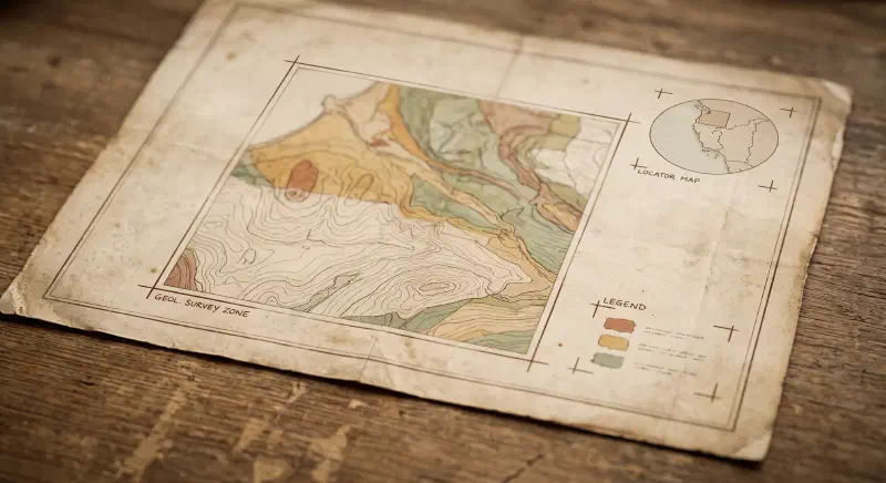
- A geological map sheet packs a title, the main map, a legend, a scale, an index map, cross-sections and a stratigraphic column into one image. Stratigraphic Amenity finds each part with a YOLOv10 detector from Microsoft’s PEACE project, then runs a second detector over the legend.
- The legend detector returns colour swatches and text boxes with no link between them. A short geometric rule pairs them, and each swatch’s colour is taken as the median of its pixels.
- The toolkit reads no text. Legend labels stay empty on purpose, and every result says so, so an agent cannot mistake a detected box for a named rock unit.
Key Takeaways
- One YOLOv10 detector, trained by Microsoft’s PEACE project, finds eight structural parts of a map sheet - title, main map, legend, scale, index map, cross-sections, stratigraphic column and other. The main map’s four corners are cropped separately, since coordinate grid labels usually sit there.
- A quiet bug in PEACE’s forked detector runtime silently drops confidence scores whenever
save,save_txt,verboseorshowis truthy - andsave_txtdefaults to true. The wrapper sets all four to false explicitly, and a test locks that in. - Legend swatches and their text are not linked by the detector - a geometric rule pairs them. The nearest text box to a swatch’s right edge is accepted only if the distance is no more than the swatch’s own height; each swatch’s colour is the median of its pixels, ignoring near-black outline pixels.
- There is deliberately no OCR, because agents filled in plausible labels when results looked complete. Every legend entry now comes back with
label: null, and area-coverage numbers are explicitly flagged as a colour heuristic, not a measurement.
A question about a geological map, such as which rock unit dominates the northeast of the sheet, depends on several parts of the sheet at once. The coloured polygon is in the main map. What the colour means is in the legend. Where the map sits on Earth depends on grid labels around the map frame. Before any of that can be read, something has to find the parts.
This post covers map layout detection and legend extraction in Stratigraphic Amenity, the open-source toolkit we built on top of Microsoft’s PEACE research.
Eight parts of a map sheet
The component detector is a YOLOv10 object-detection model trained by the PEACE project. It recognises eight classes:
| Class | What it is |
|---|---|
title | The map title |
main_map | The mapped area itself |
legend | The explanation box of colour swatches and unit names |
scale | Scale bar or ratio |
index_map | The small locator map |
cross_section | Geological cross-sections |
stratigraphic_column | The column showing unit order |
others | Anything else |
For every detection the service saves a crop of that region and records its bounding box and confidence. Two classes get extra treatment.
- Main map. Besides the crop, the service cuts out the four corners of the panel, each 10% of its width and height, and joins them into one 2 by 2 image. Coordinate grid labels usually sit in those corners, and an OCR step or vision model can read them there to produce ground control points for georeferencing.
- Index map. The crop gets a white border with compass labels (N, S, E, W and the diagonals), carried over from PEACE, so a vision model reading it knows which way is which.
All of this is drawn onto a single overview image with a coloured box per class and its confidence, alongside a metadata file in PEACE’s format.
A detail in the PEACE fork
PEACE ships its own fork of the Ultralytics runtime, and it behaves differently from the PyPI package in one way that silently drops confidence scores. In that fork, if any of the save, save_txt, verbose or show options is truthy, prediction returns a dictionary keyed by class name instead of a results object, and the dictionary carries no confidence values. The fork’s default for save_txt is true.
The detector wrapper therefore sets all four to false explicitly on every call, and a test locks that in. It is the kind of behaviour you only find by reading what comes back.
Pairing swatches with their text
The second detector runs on the legend crop and finds two kinds of box: colour swatches and text blocks. It does not say which text belongs to which swatch. The pairing is done geometrically.
For each swatch, in the order the detector returned them:
- Take the point at the swatch’s right edge, halfway down.
- For every unpaired text box, take the point at its left edge, halfway down.
- Pick the nearest text box.
- Accept the pair only if that distance is no more than the swatch’s own height. Otherwise the swatch is skipped.
The threshold scales with the legend’s own proportions. A text box that starts a few pixels to the right of an 8-pixel-high swatch is paired; one in the next column is not. Paired text boxes are then trimmed of blank margins, where a column counts as blank when its darkest pixel is still near white.
On a small synthetic test legend, a swatch at [2, 2, 10, 10] and a text box at [15, 1, 42, 11] are 5 pixels apart, under the swatch height of 8, so they pair. Both boxes are then shifted from legend-crop coordinates back into full-image coordinates.
Reading the colour
A swatch is rarely one flat colour after scanning. The service takes the median of the swatch’s pixels, ignoring near-black pixels (every channel below 16) that come from outlines and hatching. It reports the colour as RGB, as a hex code, and as the nearest of 25 basic colour names.
Estimating how much of the map each unit covers
With swatch colours known, the service estimates what fraction of the main map panel is painted in each one. For each legend colour it sets a tolerance of half the colour distance to the nearest other legend colour, so similar units get tight tolerances and distinct units get looser ones. It then counts the pixels within tolerance. Pure white entries are skipped.
This is a colour heuristic and is labelled as one. Topographic lines, printed text and units with nearly identical colours all count, and the denominator is the whole panel including blank margins. It is a hint about which units dominate, useful for deciding where to look first, and not a measured area.
What the toolkit deliberately does not do
There is no OCR in Stratigraphic Amenity. The detector finds the box a legend label sits in and does not read the words inside it. Every legend entry therefore comes back with label: null and label_extraction: "not_available", and the result text says that labels were not extracted.
We made that explicit after testing with real agents. When a result looked like a complete legend, agents filled in plausible unit names on their own. Now the count is reported as “legend_extracted_candidates: N (not a verified map-unit count)”, and the labels have to come from the caller’s own OCR or vision model, or from a person.
Two further limits are worth knowing. Only the first legend region and the first main map region are used for swatch pairing and area estimates, even on sheets with several panels. And the detector stack is pinned to CPU PyTorch wheels, so processing a large sheet takes a while.
Plugging in a different detector
The service does not depend on YOLOv10 specifically. Any object with a detect(image_path) method that returns bounding boxes per label can be passed in. The test suite uses small fake detectors this way, and the same seam lets someone swap in a detector trained on their own map series.
The layout and legend code lives in src/stratigraphic_amenity/map_processing/ in the Stratigraphic Amenity repository. Once the map frame is found, the next step is locating it on Earth, described in Georeferencing a Scanned Geological Map From Ground Control Points. For the project’s background, see Geological Map Processing Suite.