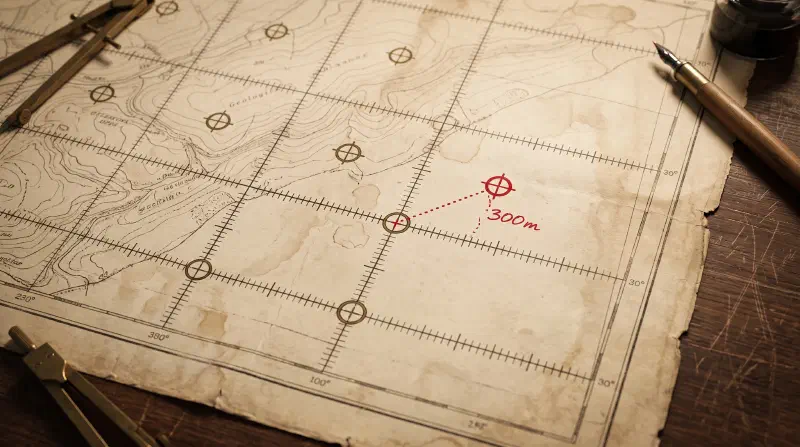
TL;DR
- A scanned map is a grid of pixels with no geographic meaning until pixel positions are tied to real coordinates. This can be done with an affine fit from ground control points (GCPs) read off the map, which is then reprojected to longitude and latitude.
- Two or three GCPs always fit exactly, so their residual is zero and proves nothing. With four or more, the fit has spare data and a leave-one-out check becomes possible.
- In our worked example, one corner coordinate misread by 300 m produced a 75 m residual spread evenly across all four points. The leave-one-out error came back at 300.03 m and exposed it.
Key Takeaways
- A perfect fit through two or three control points proves nothing. An exact fit always has a zero residual. Only four or more points give the fit spare data that can reveal a bad coordinate.
- Least squares hides a single misread point, but leave-one-out does not. One easting misread by 300 m produced an even 75 m residual and identical 2.49-pixel errors on all four points - no single point looked wrong. Predicting that point from the others instead exposed the full 300 m.
- Check orientation before trusting the numbers. On a north-up map the y scale term must be negative. A positive one usually means a northing with the wrong sign or swapped points.
- An affine fit is enough to locate a map for catalogue and database queries. Warped or folded scans would need a polynomial or spline fit, which the module does not offer.
A geological map sheet scanned to PNG or TIFF is a picture. To ask what earthquakes, faults or mineral occurrences fall inside the mapped area, a program first has to know where on Earth each pixel sits. That step is georeferencing, the geospatial process of tying image pixels to real-world coordinates.
Microsoft built the underlying toolkit for this kind of map processing, PEACE, bundled together with its own map-reading agent. Stratigraphic Amenity, our open-source toolkit for geological maps, repackages PEACE’s core operations - layout detection, georeferencing and overlays among them - into a small Python SDK and local MCP server, so any AI agent can call them directly as tools instead of going through PEACE’s own bundled agent. Georeferencing is handled in its georef module.
This post explains the method, the checks that tell you whether to trust the result, and the mistakes those checks are designed to catch.
Pixels and world coordinates run in different directions
An image has its origin at the top-left corner. x grows to the right and y grows downward. A projected coordinate system such as UTM measures easting and northing in metres, and northing grows toward the top of a north-up map.
So the two y axes point in opposite directions. On a normal map, moving one pixel down the image moves you south, and the transform has to encode that. It is also the first sanity check the module runs, covered below.
The affine transform
The module fits six numbers, a to f, that map a pixel to a world coordinate:
world_x = a * pixel_x + b * pixel_y + c
world_y = d * pixel_x + e * pixel_y + faandeare metres per pixel along each axis. On a north-up mapeis negative.banddcapture rotation and shear, and are zero for a map scanned perfectly straight.candfare the world coordinates of pixel (0, 0).
Take the example from the project README, a 1000 by 1000 pixel map in NAD83 / UTM zone 15N (EPSG:26915), with two ground control points:
- pixel (0, 0) is at easting 660000, northing 5400000;
- pixel (1000, 1000) is at easting 690000, northing 5370000.
Then a = (690000 − 660000) / 1000 = 30 metres per pixel eastward, and e = (5370000 − 5400000) / 1000 = −30, so each pixel down is 30 metres south. c and f come straight from the first point. Pixel (500, 500) lands at easting 675000, northing 5385000. Reprojected to WGS84, the map’s bounds come out at longitude −90.8356 to −90.4165 and latitude 48.4544 to 48.7325, in northwest Ontario.
Where the control points come from
A GCP is a pixel position paired with a known world coordinate, typically a grid tick with a printed label such as “660000E” at a corner of the map frame. Stratigraphic Amenity does not read those labels itself. It ships no OCR, so the coordinates come from the calling agent’s own OCR or vision model, or from a person.
To make that reading easier, the layout detection step saves a small mosaic of the four corners of the main map panel, each corner cropped to 10% of the panel’s width and height, where coordinate labels usually sit.
How many control points, and why four
The module chooses its fitting method from the number of points supplied:
| GCPs | Method | What the residual tells you |
|---|---|---|
| 1 | Rejected | Nothing can be fitted |
| 2 | Axis-aligned exact fit (scale and offset, no rotation) | Always zero. The two points must differ in both x and y |
| 3 | Exact full affine | Effectively zero. The points must not lie on one line |
| 4 or more | Least squares | Meaningful, and a leave-one-out check can run |
Two points always define a line that passes through both of them, so a perfect fit through two points is no evidence that either point was read correctly. The same holds for three points and an exact affine. Only with more data than unknowns does the fit reveal inconsistency.
The module is explicit about this. A fit from fewer than four points is flagged residual_diagnostic: false and comes with the warning residual_not_diagnostic: an exact fit has no independent error check; supply at least 4 well-distributed GCPs.
What the result reports
georeference_bounds returns more than a bounding box:
- residual, the root-mean-square error of the fit in the map’s own units;
- residual_m, the same error measured geodesically in metres on the WGS84 ellipsoid;
- gcp_pixel_errors, how far each world coordinate lands from its pixel when run back through the inverse transform;
- holdout_error, available from four points up, the worst error when each point in turn is left out of the fit and then predicted;
- warnings about the shape of the transform.
The warnings check orientation. a at or below zero flags a nonstandard x direction. e at or above zero flags a nonstandard y direction, which on a north-up map usually means a northing was typed with the wrong sign or the points were swapped. A cross term larger than 10% of the scale terms flags substantial rotation or shear.
Catching a misread coordinate
Here is why the leave-one-out figure matters. We ran the same four-corner fit twice.
Four clean points. Least squares, residual about 7 micrometres (floating-point noise), leave-one-out error about 16 micrometres, no warnings.
Four points with one misread. One corner’s easting was entered as 690300 instead of 690000, a 300 m error of the kind a misread digit produces.
residual         = 75.0 m
gcp_pixel_errors = [2.49, 2.49, 2.49, 2.49]
holdout_error    = 300.03 m
Least squares spreads one bad point’s error across all the points. Every point looks 2.49 pixels off, so the per-point errors cannot tell you which one is wrong, and a 75 m residual on a regional map might pass without comment. The leave-one-out error does not dilute. When the bad point is held out and predicted from the other three, it misses by the full 300 m.
The practical rule follows. When holdout_error is much larger than residual_m, suspect a single misread point, and find it by refitting with each point removed in turn.
Limits of an affine fit
- Affine only. Scans that are warped, folded or stretched unevenly cannot be fitted exactly. There is no polynomial or thin-plate spline option.
- Bounds from four corners. The longitude and latitude box is computed from the corners of the map panel. Over very large extents, the edges of a projected frame can bow slightly outside that box.
- Maps that cross the antimeridian produce one enormous box from −179 to 179 instead of two pieces. The knowledge query layer has a separate entry point that splits such extents.
- North-up assumptions appear in other places, such as drawing results back onto the map image.
For locating a map well enough to query earthquake catalogues and fault databases around it, those limits rarely matter. For precise digitisation they would.
Reading the coordinate system off the map
Maps usually print their coordinate system as free text, such as “UTM N83 Zone 15”. Before the fit can be reprojected to longitude and latitude, that text has to become a code a projection library understands - a coordinate reference system (CRS) identifier such as EPSG:26915 here. The same georef module handles that step in crs.py.
The georeferencing code is in src/stratigraphic_amenity/georef/ in the Stratigraphic Amenity repository. For the project’s background and its relationship to Microsoft’s PEACE research, see Geological Map Processing Suite.