Key Takeaways
- State of the art: Continual learning methods typically treat forgetting as damage to prevent through full history accumulation, experience replay buffers, or weight-importance penalties, assuming that any training example dropped from the buffer is permanently lost to the policy.
- Unresolved problem: In iterative agent self-training, accumulating every successful trajectory scales the training buffer linearly with diminishing returns per row, whereas curating the three historically highest-scoring generations (Katalin in Survival is the Only Reward) fragments strategy space and collapses at late generations (
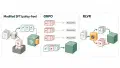
v12tov13). - When working on self-retraining using sliding window data LoRAs that finetune agents on different segments of their own prior experience, we created three experimental model lineages: one trained on all of the agent’s prior experiments, both good and bad (Terese), one on 3000 lines of data from the best three runs (Katalin) and on on 3000 lines from the most recent three runs (Miri).
- Candidate mechanism and scope: In an active environment such as our Negative Space Learning (NSL) sandbox, useful skills are re-executed by the current policy and re-enter the sliding window as fresh trajectories. While this was a limited test, it suggests a mechanism similar to the way in which humans retain the skills they use most, by simply retraining repeatedly on the most recently used capabilities.
TL;DR
When fine-tuning an LLM coding agent across multiple generations on its own successful trajectories, you must choose which historical datasets feed each update: accumulate all past generations (as we tried in our Terese lineage), select the three historically highest-scoring generations (our Katalin lineage), or keep a sliding window of the last three generations (our Miri lineage). In a 13-generation case study on Qwen2.5-7B-Instruct (Survival is the Only Reward), peak-score curation collapsed at v12 to v13, whereas the \(K=3\) recency window improved steadily without replaying older agent trajectories, reaching 14,938 MB freed per held-out run (58.4% of full accumulation’s 25,570 MB) and 2.049 offline cumulative composite score (52.6% of full accumulation’s 3.898, or 2.1× the composite-score units per training row) on a capped 15,000-row buffer.
1. The Buffer Design Question and Core Definitions
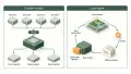
In standard continual learning, a model trains sequentially on a passive external stream of tasks where dropping old examples risks catastrophic forgetting. Standard remedies fall into two families:
- Weight regularization: Methods such as Elastic Weight Consolidation (EWC) penalize updates to parameters that mattered for earlier tasks.
- Rehearsal and coreset buffers: Methods such as Gradient Coreset Replay (GCR) store and replay a representative subset of past data alongside new examples.
An agent in an environment-mediated self-training loop operates under different dynamics. Following the framework introduced in Generalising from Self-Produced Data, the agent actively generates new candidate trajectories every round, and the environment filters them through a deterministic survival check before the next fine-tune.
Operational Definitions (Episode, Row, Generation, and Fresh LoRA Reset)
To make the experimental comparison and row accounting unambiguous, here is how each object is defined in the study:
- Episode (run) and binary survival gate \(\mathcal{S}(\tau) \in \{0, 1\}\): In one episode of
scripts/main.py, the agent interacts with a network of disposable Alpine Linux containers (docker/special-learn-compose) across three stages: (1) environment discovery, (2) cleanup strategy listing, and (3) Python execution, with up to three error-correction retries per stage. Before and after the episode, the harness measures available disk space across the containers viadf -k /.- Passing trajectory (\(\mathcal{S}(\tau)=1\), \(\Delta R(\tau) > 0\)): The agent scans the container network, identifies seeded junk archives in
/tmp/cleanupor/var/cache, and removes them over SSH without breaking container viability, increasing net available storage. - Failing trajectory (\(\mathcal{S}(\tau)=0\), \(\Delta R(\tau) \le 0\)): The script errors out across all retries, times out, or executes valid commands that free zero net bytes; the episode is logged for audit but excluded from SFT export.
- Passing trajectory (\(\mathcal{S}(\tau)=1\), \(\Delta R(\tau) > 0\)): The agent scans the container network, identifies seeded junk archives in
- Training row: One prompt-completion pair exported from a passing episode for supervised fine-tuning (standard next-token cross-entropy loss on assistant completion tokens, with prompt tokens masked via
IGNORE_INDEX = -100). Because one passing episode includes discovery, strategy, and execution turns, each successful episode contributes multiple training rows until the generation reaches its quota of4,500agent-generated rows. - Generation (
v1tov13) and the fresh-LoRA lifecycle:v1is the untouchedQwen2.5-7B-Instructbase model, which executes episodes to produce Dataset1. Every later model checkpointv_t(v2throughv13) is produced by training a fresh QLoRA adapter (rank=32,alpha=32, 4-bit NF4, learning rate2e-4, 3 epochs) directly on the frozenv1base model using a selected subset of prior datasets, andv_tthen collects Datasett:
Checkpoint v_{t-1} acts in sandbox -> Survival gate (ΔR > 0) keeps 4,500 agent rows (Dataset t-1)
  -> Regime rule selects prior datasets + 500 rehearsal rows per dataset
  -> Fresh QLoRA adapter trained from frozen Base Model (v1) -> Produces Checkpoint v_t
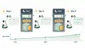
Why call this continual learning if weights reset to v1 every round? Because adapters are never stacked on v_{t-1}, no weight drift compounds across generations; instead, continual learning happens through the closed-loop data channel. If an agent discovers and trains on a useful skill during generation 1, it will most likely repeat it in generation 2 and 3, meaning that it stays in future training sets long after the generation 1 dataset has been discarded. Conversely, if environments change and the skill is no longer useful, the agent will use it less frequently and it will gradually disappear from future training datasets.
Worked Illustration: How a 3-Generation Window Retains or Drops Skills
Suppose across five generations an agent discovers strategy A (clearing /tmp caches) in v1, refines A and discovers B (SSH cleanup on the peer container) in v2, and discovers C (compressing logs) in v3. As long as A and B remain effective in v4 and v5, the current policy keeps executing them, so fresh trajectories implementing A, B, and C populate Datasets 3, 4, 5. When v6 trains only on Datasets 3, 4, 5, it retains A and B without needing Dataset 1 or 2 in storage. Conversely, if the environment changes at v4 so that A no longer frees space, A stops passing \(\mathcal{S}(\tau)=1\) and ages out of the buffer by v7, illustrating both how the window prunes obsolete habits and why it cannot protect a skill that goes unused for \(K\) consecutive generations.
2. The Three Buffer Regimes, Row Accounting, and Evaluation Protocol
In Survival is the Only Reward, three lineages started from identical Qwen2.5-7B-Instruct base models, ran the same accumulation pipeline for a five-generation warm-up (v1 to v5, Datasets 1..4), and then diverged from v6 through v13 under three dataset-selection rules:
| Regime (Lineage Name) | Selection Rule for Checkpoint v_t (\(t \ge 6\)) | Datasets Used at v13 | Agent Rows at v13 | Fixed Rehearsal Rows at v13 | Total Trainer Rows at v13 | Optimizer Examples (3 Epochs, Capped at 17,000 in Annex II) |
|---|---|---|---|---|---|---|
| Full History (Terese) | All prior datasets 1..t-1 | 1..12 (12 datasets) | 54,000 | 6,000 (500 × 12) | 60,000 (100%) | Scaled with buffer (up to Annex II cap) |
| Sliding Window \(K=3\) (Miri) | Last 3 datasets {t-3, t-2, t-1} | 10, 11, 12 (3 datasets) | 13,500 | 1,500 (500 × 3) | 15,000 (25%) | Fixed 3-dataset window per round |
| Top-3 Historical (Katalin) | Top 3 prior datasets by online code-run success % | 8, 10, 11 (3 datasets) | 13,500 | 1,500 (500 × 3) | 15,000 (25%) | Fixed 3-dataset window per round |
Rehearsal accounting: Each generation’s dataset (5,000 rows) consists of 4,500 self-generated trajectory rows collected via scripts/data_collector.py plus a fixed 500-row general-text slice from the Stack Exchange Paired dataset (chosen because it predates the base model’s training corpus). Because 500 rehearsal rows are bundled per dataset, the 15,000 vs. 60,000 trainer-row ratio (25%) is identical whether counted on agent-generated rows (13,500 / 54,000 = 25%) or total trainer rows (15,000 / 60,000 = 25%).
How the Raw Metrics and Standardized Composite Score Are Calculated
Early generations required 5 to 7 days of wall-clock runtime to collect 4,500 passing rows, whereas later generations finished in 10 to 15 hours. Because raw wall-clock hours depend on GPU thermal state and host load, the paper tracks two storage-outcome metrics per checkpoint \(i \in \{1, \dots, 13\}\):
- \(P_i\) (% of total space freed): Fraction of total available container space captured.
- \(A_i\) (Average space taken over per run, in MB): Mean storage freed per episode, serving as a per-episode efficiency measure. (General code compilation accuracy is tracked separately in Table 9 and excluded from the composite score because agents learned to issue deliberately failing probe scripts to harvest error messages.)
To combine \(P_i\) and \(A_i\) on a common scale (scripts/unweighteddeltas.py), each metric’s step-over-step change from checkpoint \(i-1\) to \(i\) is divided by that metric’s standard deviation \(\sigma\) across the lineage’s 13 checkpoints (v1..v13), and accumulated from v1 (anchored at 0.000):
Because \(\text{Cumulative Score}_t\) is a running sum of signed standardized step changes, positive transitions add to the total and regressions subtract from it. For example, in Terese’s online run (Table 2), v1 starts at 0.000, v2 gains +1.951 (cumulative 1.951), v3 gains +0.674 (cumulative 2.624), and v4 regresses by -0.239 (cumulative 2.385).
Online vs. Offline Evaluation Protocol
Every checkpoint v1 through v13 is measured two ways:
- Online metrics (Tables 2, 4, 6): Recorded across the live data-collection run required to gather
4,500passing rows for the next generation. This reflects path-dependent performance while the agent populates its next training buffer. - Offline held-out metrics (Tables 3, 5, 7): Recorded across three independent 100-episode evaluation runs (
3 × 100episodes) generated by the same procedural container-seeding code (variation_1throughvariation_5templates) but completely held out from training. Offline tables report the mean and 95% confidence interval (n = 3evaluation runs per checkpoint).
3. Results: Raw Outcomes and Composite Scores Across 13 Generations
Scope and Experimental Limits (Read Before the Table)
- Single lineage per regime: Each regime (Terese, Miri, Katalin) was run as a single 13-generation lineage on one task and one base model (Qwen2.5-7B-Instruct), with additional offline testing to establish error bounds. The 95% confidence intervals in the offline tables measure variance across the 3 held-out evaluation runs of that checkpoint, not variance across multiple independent training seeds.
- Data efficiency, not compute efficiency: All three regimes run the same
4,500-row data-collection loop every generation. The 4× savings in Miri (15,000vs.60,000rows atv13) measure training-buffer row efficiency, not measured wall-clock training GPU-hours or total pipeline compute. - Single window size (\(K=3\)): The experiment tested \(K=3\) after a 5-generation warm-up and did not sweep \(K\).
Endpoint Comparison (v1 Baseline vs. v13 Final Checkpoint)
Tables 2 through 7 of Survival is the Only Reward report both the raw storage outcomes and the standardized composite scores:
| Regime | Held-Out Offline % Space Freed (v1 \(\to\) v13) | Held-Out Offline Avg MB / Run (v1 \(\to\) v13) | Online % Space Freed (v1 \(\to\) v13) | Online Avg MB / Run (v1 \(\to\) v13) | Offline Cumulative Composite Score at v13 | Online Cumulative Composite Score at v13 | Offline Composite Units per Row (Terese = \(1.0\times\)) |
|---|---|---|---|---|---|---|---|
| Full History (Terese) | 3.1% ± 1.4% \(\to\) 16.6% ± 0.9% | 5,211 ± 2,275 \(\to\) 25,570 ± 914 | 2.5% \(\to\) 16.9% | 3,678 \(\to\) 23,758 | 3.898 ± 0.927 (100%) | 3.109 (peak 3.728 at v7) | 1.00× |
| Sliding Window \(K=3\) (Miri) | 3.4% ± 1.8% \(\to\) 9.0% ± 1.9% (54.2% of Terese) | 5,697 ± 2,874 \(\to\) 14,938 ± 3,240 (58.4% of Terese) | 3.4% \(\to\) 12.0% | 5,703 \(\to\) 16,223 | 2.049 ± 1.602 (52.6% of Terese) | 3.322 | 2.10× |
| Top-3 Historical (Katalin) | 3.4% ± 1.8% \(\to\) 9.0% ± 1.9%* | 7,293 ± 479 \(\to\) 9,506 ± 2,165 (37.2% of Terese) | 4.5% \(\to\) 4.5% (peak 13.9% at v11) | 6,549 \(\to\) 6,349 (peak 20,943 at v5) | 0.482 ± 0.675 (12.4% of Terese) | -0.008 (collapsed) | 0.49× |
(Data note on Katalin Table 7: In the arXiv PDF, the “Mean of % space freed column of Table 7 inadvertently duplicates Miri’s Table 5 values. The correct offline means are plotted in Figure 3: Katalin’s space freed rises to =11.6% at v1ø and =10.5% at v11, then falls to ~5.8% at v12 and =5.7% at v13. Table 6’s online column shows the same collapse, from 13.9% at v11 to 6.2% at v12 and 4.5% at v13. So do Table 7’s own “Mean of average space taken over per run (MB)” and “Mean cumulative composite improvement score” columns, from 17,491 MB and 2.233 at v11 to 9,506 MB and 0.482 at v13 )
Four Findings From the Data
- Raw outcomes and composite scores tell the same efficiency story for Miri: On one-fourth of Terese’s
v13training rows (15,000vs.60,000), Miri’sv13checkpoint captures58.4%of Terese’s held-out MB per run (14,938vs.25,570 MB),54.2%of Terese’s held-out % space freed (9.0%vs.16.6%), and52.6%of Terese’s offline cumulative composite score (2.049vs.3.898). Dividing offline composite score byv13trainer rows gives \((2.049 / 15,000) / (3.898 / 60,000) = 2.10\times\) as many composite-score units per row (or \(2.34\times\) in held-out MB per row), with overlapping 95% evaluation confidence intervals between Miri (2.049 ± 1.602, peaking at2.550 ± 1.518atv9) and Terese (3.898 ± 0.927). - Full accumulation (Terese) achieves the highest absolute ceiling, with diminishing per-row returns: Keeping all
60,000rows yields the highest held-out storage capture (16.6%,25,570 MB/run). However, Terese reaches2.834 ± 1.868offline (20,089 MB/run) byv4on15,000rows; the remaining45,000rows added acrossv5..v13buy the final+1.064composite score units. - Top-3 peak selection (Katalin) climbs early and collapses at
v12..v13: Katalin’s selector ranks prior generations by the online percentage of code blocks that compiled and ran cleanly (Table 9). After rising throughv5(2.913online,1.603offline) and holding throughv11(2.624online,2.233offline on Datasets8, 9, 10), locking onto the disconnected historical trio8, 10, 11atv12andv13triggers a sharp regression: online MB/run falls from17,114 MB(v11) to8,647 MB(v12) and6,349 MB(v13, belowv1’s6,549 MB), and offline MB/run drops from17,491 MBto9,506 MB. - Reported transfer checks (HumanEval and Windows Docker): Rather than a full multi-domain forgetting benchmark, the paper reports two targeted checks. On HumanEval (Table 8, evaluated in a single pass with an automated script stripping markdown backticks and comments to match the agent harness), Pass@1 / Pass@4 shifts modestly from base
Qwen2.5-7B-Instruct(77.59% / 85.37%) tov13(75.61% / 81.71%for Terese;74.09% / 82.32%for Miri;74.24% / 79.88%for Katalin). On a single-pass evaluation in a Windows-based Docker container environment running the same storage-recovery task (Table 11), baseQwen2.5-7B-Instructfreed3.63%(6,117 MB/run), whereas Miriv13freed8.19%(13,651 MB/run) and Teresev13freed15.67%(23,756 MB/run).
4. Observed Diagnostics vs. Candidate Mechanisms
To keep empirical measurements separate from causal interpretation, we group Section 7 of our NSL paper into three levels of evidence:
- [Observed in PCA strategy maps] Subtractive pruning of strategy variance \(D_t\): In Section 7.2 of the paper, each generated strategy string \(y\) is projected into a token-embedding PCA space \(\phi(y) \in \mathbb{R}^d\) with generation centroid \(\mu_t = \mathbb{E}_{y \sim \pi_{\theta_t}}[\phi(y)]\) and strategy-embedding variance \(D_t = \mathbb{E}_{y \sim \pi_{\theta_t}}\!\left[\|\phi(y)-\mu_t\|^2\right]\). Across Figures 6 to 8 and 12 to 14, Negative Space Learning exhibits declining \(D_t\) from
v1tov13: rather than inventing unbounded new clusters, agents compress probability mass into tighter basins of repeatable strategies. - [Observed in pass@1 vs. compile-rate divergence] Instrumental debugging probes: In Tables 9 and 10, overall code compilation-and-run rates climb from
20.9%..33.2%atv1to57.9%..85.5%atv13, while first-attemptpass@1drops to0.00%online for Terese and Katalin fromv6onward (0.36%for Miri atv13). Agents converged without instruction on using early retry turns to run fast diagnostic probes whose error messages guide the final cleanup script. - [Candidate hypothesis] Endogenous replay via the environment in Miri: Unlike generative replay methods that train an auxiliary generator to synthesize old data (Krawczyk et al., 2024), Miri relies on the policy re-executing strategies that still work in the current container state so they re-enter
{t-3, t-2, t-1}. While the basin-persistence plots (Figure 13) are consistent with strategy reuse, the study did not track exact per-strategy recurrence rates across windows, leaving endogenous replay a plausible mechanism rather than a causally isolated proof. - [Candidate hypothesis] Modal fragmentation in Katalin: Why did training on Datasets
8, 10, 11collapse atv12..v13? Because each round starts from a fresh LoRA onv1, training on high-scoring datasets from non-adjacent historical generations (8, 10, 11) may pull the adapter simultaneously toward incompatible behavioral modes optimized for different stages of the lineage. However, without multi-seed reruns or controlled dataset-swap ablations on Katalin’sv11state, we cannot rule out simpler explanations such as sample-mix noise or a single anomalous generation.
In contrast to passive task streams mapped in continual learning surveys, this self-generating window only protects skills that the environment continues to exercise.
5. Try It Yourself: Two Codebases and How to Run a \(K\)-Sweep
Our workspace includes two repositories that correspond to two stages of this research. Distinguishing them up front avoids confusion between the paper’s exact setup and our current framework:
- Original Experiment Repo (Public,
EigenformAI/Negative-Space-Learning,HEAD 684e28b): Contains the 3-stage Alpine container sandbox (docker/special-learn-compose), the episode runner (scripts/main.py), the bulk collector (scripts/data_collector.py), and the composite-score template (scripts/unweighteddeltas.py), plus DPO pairing scripts (scripts/create_DPO_dataset.py,scripts/train_DPO.py). The SFT training hyperparameters used for Terese, Miri, and Katalin onQwen/Qwen2.5-7B-Instructare listed in Annex II of the paper (pages 36 to 37: 4-bit NF4,lora_rank=32,lora_alpha=32,model_max_length=1024,max_examples=17000,num_train_epochs=3,per_device_train_batch_size=1,gradient_accumulation_steps=32,learning_rate=2e-4, cosine schedule). - Current Unified Framework (
NSL2,HEAD bd2faae): Replaces the standalone scripts with an automated multi-generation generate-then-train orchestrator (scripts/run_train_loop.py), a QLoRA/DFT/ASFT trainer (src/train/qlora.py), and a task contract (tasks/memory_cleanup.py).
How NSL2 Implements the Trailing Window (0-Indexed Generations)
In NSL2 (scripts/run_train_loop.py:699-789), generations are 0-indexed (generation_0 through generation_{num_gens-1}). In iteration generation_id, the current model first completes data collection and exports its SFT rows to generation_<generation_id>/exports/sft/latest.json. Immediately after that generation completes, _collect_training_window_paths (:167-180) gathers the trailing window_size completed directories, from max(0, end_generation_id - window_size + 1) through end_generation_id inclusive, to train the fresh adapter after_generation_<generation_id> for the next round:
# scripts/run_train_loop.py:167-180 (NSL2, commit bd2faae)
def _collect_training_window_paths(
    generation_root: Path,
    end_generation_id: int,
    window_size: int,
) -> list[Path]:
    if window_size < 1:
        raise ValueError("training window size must be positive")

    start_generation_id = max(0, end_generation_id - window_size + 1)
    training_paths: list[Path] = []
    for generation_id in range(start_generation_id, end_generation_id + 1):
        generation_dir = generation_root / f"generation_{generation_id}"
        training_paths.append(resolve_latest_sft_training_rows_path(generation_dir))
    return training_paths
Here generation_0 (collected by the untouched base model, equivalent to v1 writing Dataset 1 in the paper) produces adapter after_generation_0 (equivalent to v2). With num_generations = 13 (generation_0 through generation_12), training runs after each of the first 12 generations (generation_0..11), and generation_12 is the final evaluation generation (equivalent to v13 trained on up to 12 prior datasets).
Configuring Miri, Terese, and a \(K \in \{1, 3, 5\}\) Sweep in NSL2
The shipped config/config-memory-cleanup-msagent.toml defaults to a smaller 5-generation run on Qwen2.5-Coder-7B-Instruct (target_training_rows = 2000). To align the config with the 13-generation Qwen2.5-7B-Instruct window comparison, override [generation], [training], and [orchestration]:
# Adapted from config/config-memory-cleanup-msagent.toml
model_name = "vllm:Qwen/Qwen2.5-7B-Instruct"

[generation]
target_training_rows = 4500
generation_output_dir = "./data/miri-k3/generations"

[training]
base_model = "Qwen/Qwen2.5-7B-Instruct"
max_seq_length = 1024
num_train_epochs = 3
per_device_train_batch_size = 1
gradient_accumulation_steps = 32
learning_rate = 2e-4
lr_scheduler_type = "cosine"
warmup_ratio = 0.03
lora_rank = 32
lora_alpha = 32
adapter_output_dir = "./models/adapters/miri-k3"
rehearsal_dataset = "HuggingFaceH4/stack-exchange-preferences"
rehearsal_rows_per_epoch = 500

[orchestration]
num_generations = 13
training_window_size = 3 # Miri: 3 | Terese: 12 (or >=12) | Sweep: 1, 3, 5- Run the loop:
uv run python scripts/run_train_loop.py --config config/your-config.toml(giving each regime its owngeneration_output_dirandadapter_output_dir). - Compare across \(K \in \{1, 3, 5\}\) and multiple seeds: Set
training.seed(e.g.,42, 43, 44) and summarize per-generationsuccess_rate,training_row_count, andtraining_data_pathsacross runs withuv run python scripts/analyze_metrics.py.
FAQs
What is a training row in sliding window SFT, and do the 15,000 vs. 60,000 counts include rehearsal data?
Each passing episode exports its prompt-completion turns as supervised fine-tuning rows (4,500 agent-generated rows per generation), supplemented by 500 fixed Stack Exchange rehearsal rows (5,000 total trainer rows per generation). At v13, a 3-generation window trains on 13,500 agent rows plus 1,500 rehearsal rows (15,000 total), while 12-generation full accumulation trains on 54,000 agent rows plus 6,000 rehearsal rows (60,000 total), so the 25% data ratio holds under both counts.
What does “52.6% of full-accumulation offline gains” actually measure?
It is the ratio of the standardized cumulative composite improvement scores at v13 (2.049 for Miri vs. 3.898 for Terese), where each generation’s change in % space freed and average MB captured per run is normalized by its standard deviation across checkpoints. On the underlying raw held-out metrics at v13, Miri reaches 58.4% of Terese’s average MB captured per run (14,938 MB vs. 25,570 MB) and 54.2% of Terese’s % space freed (9.0% vs. 16.6%).
Why is this called continual learning if every generation resets to a fresh LoRA adapter on the base model?
Instead of sequentially updating one shifting set of weights (which compounds drift across generations), each round fits a fresh LoRA adapter on the frozen v1 base model using the current data window. Competence accumulates across generations through the data channel: adapter v_{t-1} executes stronger strategies in the environment, writing higher-yield trajectories into the buffer that trains v_t.
Does this experiment prove sliding window SFT prevents catastrophic forgetting in general?
No. The study ran one 13-generation lineage per regime on one container task and one base model (Qwen2.5-7B-Instruct). Within that scope, dropping generations older than \(K=3\) caused no monotonic collapse on the task and only a small shift on a single-pass HumanEval check (77.59% to 74.09% Pass@1), but the window only preserves skills that the agent continues to exercise in its environment.