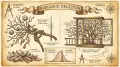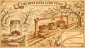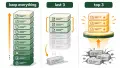
Key Takeaways
- State of the art and curriculum learning: Conventional data selection self-improvement (such as Best-of-N and rejection sampling) treats top-performing trajectories as gold-standard supervision, assuming that curating peak reward functions like an effective curriculum learning filter in stationary environments.
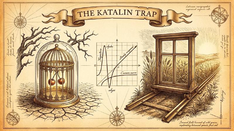
- The Katalin Trap and self-training collapse: In agentic non-stationary tasks, cherry-picking training data can cause niche overfitting and self-training collapse, as happened in the case of the “Katalin” experiment described below.. Because successful actions permanently consume the environment’s exploitable state, peak trajectories represent transient exploits from dead worlds rather than robust generalisation.
- Non-parametric catastrophic forgetting: Unlike classical catastrophic forgetting caused by weight interference, the rise-and-collapse failure mode in our Negative Space Learning experiments occurs under frozen base models with fresh LoRA adapters, driven entirely by discarding recovery and exploration behaviours.
- Sliding window training and online stability: Retaining recent trajectories regardless of score acts as a temporal anchor and biological respiratory rhythm. A sliding window training buffer preserves messy recovery behaviours and forces continual re-derivation, sustaining long-term online learning stability.
TL;DR
Filtering for peak performance seems like it should be an obvious choice in data selection for self-improvement, but cherry-picking training data in dynamic environments can causes catastrophic self-training collapse. In our Negative Space Learning experiments, an agent trained only on its highest-scoring runs (Katalin) suffered niche overfitting to depleted states, unlearning its gains within eight generations without weight-level catastrophic forgetting. Conversely, sliding window training across recent generations (Miri) discards stale strategies and preserves recovery behaviours, achieving superior online learning stability on four times less data.
The Search Question
You did everything right. You ran your self-training loop, collected trajectories, and filtered for the best ones: the runs where your agent performed spectacularly. Best-of-N, rejection sampling, cherry-picking training data from the winners. Conventional wisdom says this is how you get a better model.
Why would selecting best-performing self-training data cause self-training collapse?
This is the question we arrived at after doing everything the playbook recommends and watching it burn. It’s sharper than asking whether rejection sampling hurts long-horizon agents, or why a self-improving agent degrades over generations. Those are symptoms. This one isolates the cause: selection.
The Negative Space Learning experiments give us a clean controlled comparison. Three lineages, same base model (Qwen 2.5 7B Instruct), same environment, same data collection pipeline. The only variable is which data you train on:
- Terese: all accumulated data. Plateaus.
- Miri: last three generations, regardless of performance. Improves steadily, with no data scaling.
- Katalin: top three performing generations. Collapses.
Katalin’s online composite score climbs from 0.000 at v1 to 2.913 by v5: a trajectory that looks like a self-improvement success story. Then it falls. By v13, the cumulative score is −0.008. The model has spent eight generations unlearning everything it gained, ending up worse than where it started. Miri, trained on the same quantity of data but selected by recency rather than performance, reaches 3.322 by the same point.
The difference is not data volume. All three lineages use roughly the same number of rows per generation. The difference is what the data represents. Katalin’s training set is a curated portfolio of peak performances: the runs where the agent freed the most disk space, executed the cleanest strategies, hit the highest numbers. Miri’s training set is just whatever happened in the last three runs, including the mediocre ones, the partial successes, the runs where the agent fumbled around and eventually got something working.
The blog post accompanying the paper describes the result plainly: Katalin’s later models were “like organisms hyper-selected for life in a particular niche but were unable to adapt to environmental change.”
That’s the core finding. When you select for peak performance in a self-training loop, you trigger niche overfitting, producing agents hyper-fit to a niche that ceases to exist the moment they finish training on it. The “best” run is optimal for the specific state of the environment at generation n. By generation n+1, that environment is gone: the easy disk space has been freed, the low-hanging strategies have been exhausted, and the agent faces a world its training data never described.
This is not catastrophic forgetting in the traditional sense. Katalin doesn’t forget old tasks; it collapses within the same task. The failure mode is closer to what Lin (2026) calls “rise-and-collapse”: pass@1 peaks within tens of gradient steps and then falls back, sometimes to near zero. The model finds a trick that works, milks it until the trick stops working, and has forgotten how to solve the actual problem. Katalin does this by construction: it selects the trick and discards everything else.
The rest of this post unpacks why. We’ll look at what “best” actually means in a non-stationary environment, why the sliding window works as a temporal anchor rather than just a memory-saving trick, and what this implies for anyone running a Best-of-N SFT pipeline on agents that operate in worlds they change by acting in them.
Assumptions & Nuance
Three assumptions make cherry-picking training data feel obviously correct. Each one is defensible in a stationary world. The NSL environment is not stationary.
Assumption 1: The best-performing data is the gold standard
Rejection sampling, Best-of-N, RLHF curation: these are the load-bearing walls of modern post-training. You generate candidates, you score them, you keep the winners. The premise is that high performance under the selection metric signals high capability. In a fixed environment, this functions like an effective curriculum learning filter where a trajectory that solves a math problem well will solve similar math problems well.
In a non-stationary environment, the premise inverts. Peak performance often reflects a transient exploit, not a robust capability. The NSL paper formalises this: a strategy’s reward ΔR depends on the environmental state E_t, and a strategy exhibiting high ΔR at time t may become ineffective at t’ > t if it exploits conditions that no longer hold. The agent that frees the most disk space in generation 5 is the agent that found the largest cache file: a file that, once deleted, does not come back. Training the next generation on that trajectory teaches it to look for a cache file that has already been deleted.
Call this temporal fraud. The selection metric records a score that was real at the time, but the score was earned by exploiting a feature of the environment that the agent’s own action destroyed. The best run is the least generalisable run, because the best run is the one that most thoroughly consumed the resource that made it possible. Katalin’s v5 peak of 2.913 cumulative composite score is a portrait of a world that vanished the moment the training data was written.
Assumption 2: “Model collapse” means synthetic-data mode collapse
When Shumailov et al. described model collapse, they identified a specific mechanism: models trained recursively on their own outputs lose tail diversity, because each generation of synthetic data narrows the distribution, and the tails (the rare, informative examples) vanish first. The fix is to mix in real data, or to regularise toward the original distribution. The diagnosis is distributional; the prescription is anchoring.
The collapse Katalin exhibits is not this. Rather than catastrophic forgetting caused by weight interference, the collapse stems from behavioral variance deletion. Katalin’s training data is not synthetically narrowed in the distributional sense; it is behaviourally overfit. The strategies in Katalin’s training set are diverse, real, executed, and environmentally validated. The problem is not that they lack variety. The problem is that they are selected for peak performance under environmental conditions that no longer obtain, and that they lack the behavioural continuity (the recovery moves, the debugging cycles, the partial successes) that make strategies recombinable across changing conditions.
The NSL paper describes this as a fragmentation of the model’s internal strategy space: “individually effective behaviours are retained, but the lower-level competences and connective tissue required to recombine them in novel situations are progressively eroded.” Once that integrative substrate is weakened, further fine-tuning drives continued divergence rather than recovery.
Same word, different mechanism. If you diagnose Katalin’s collapse as Shumailov-style mode collapse, you reach for distributional fixes: more data, more variety, a KL anchor to the base model. Some of these might help incidentally, but they don’t address the core failure. The core failure is that the training set is a museum of peak performances from dead environments. You don’t fix a museum by making it larger. You fix it by replacing the exhibits with living data.
Assumption 4: Filter for consistent high-performers
If you can’t trust a single peak run, the next move is to filter for consistency: keep the runs that perform well repeatedly. This is the logic behind top-k selection over multiple generations: don’t chase the outlier, chase the reliably good.
Katalin’s selection rule does exactly this. It retains the top three performing datasets across the entire history, regardless of recency. If a strategy performed well in generations 4, 5, and 8, Katalin keeps all three. The selection is not impulsive; it is cumulative.
The result is still collapse. By v13, Katalin’s cumulative composite score is −0.008. The consistently high-performing data is consistently high-performing in the environments where it was generated: environments that are gone.
Meanwhile, Miri retains the last three runs regardless of performance. This means Miri’s training set includes mediocre runs, partial successes, and runs where the agent fumbled. The NSL paper notes that Miri’s sliding window works as “a slow-but-effective triage mechanism, discarding less frequently-used strategies and maximising for generalisability across generations.” But the mechanism is subtler than triage. The mediocre runs carry something the cherry-picked top runs systematically discard: recovery behaviours.
The pass@1 data makes this concrete. By generation 6, all three lineages have pass@1 rates at or near zero. The agents have learned to deliberately write failing code on the first attempt, using the debug cycle as an exploration channel: eliciting informative error messages that inform subsequent attempts. This is meta-learning: the agents discovered that immediate correctness is not the objective; information acquisition is. The trajectories where the agent fails, debugs, and recovers are the trajectories that encode this meta-learning. They are also, by definition, not the trajectories that score highest on the raw performance metric.
Katalin’s top-three filter removes them. The runs where the agent fumbled and recovered score lower on space-freed-per-run than the runs where the agent executed a clean strategy first time. But the clean-strategy runs are brittle: they encode a specific trick that worked in a specific environment. The fumble-and-recover runs encode something transferable: how to diagnose a failure, how to pivot, how to extract information from an error message. Variance is not noise to be filtered. It is the substrate of adaptability. Miri keeps it because Miri doesn’t know any better. Katalin discards it because Katalin knows exactly what it wants, and what it wants is the thing that kills it.
What a Reader Will Need to Know Before Starting
Before we go further, three pieces of vocabulary.
The self-training loop. An agent (a Qwen 2.5 7B Instruct model with a freshly trained LoRA adapter) is dropped into a procedurally generated Linux container environment. It writes code, executes it, and either frees up disk space or doesn’t. The runs where it succeeds are recorded as training data. A new LoRA is then trained on a subset of that data and applied to the same frozen base model. The new adapter replaces the old one. The agent goes back into the environment. Repeat.
Each pass through this loop is a generation. The full sequence of generations (v1 through v13) sharing the same base model and the same data-selection rule is a lineage. The lineages do not share parameters: each generation gets a fresh LoRA trained from scratch on the base model, not stacked on the previous adapter. Inter-generation continuity comes entirely through the data, not through the weights.
The three lineages. The NSL paper runs three:
- Katalin: each generation trains on the top three datasets by performance, selected across the entire history. If generation 4, 5, and 8 had the highest scores, Katalin v13 trains on data from those three, regardless of how recent they are. This is cherry-picking by design.
- Miri: each generation trains on the last three datasets, regardless of score. Miri v6 trains on data from v3, v4, and v5; Miri v7 on v4, v5, and v6. A sliding window of recency, nothing more.
- Terese: each generation trains on all accumulated data. Terese v2 has 5,000 rows, v13 has 60,000. This is the data-scaling baseline. It plateaus. We mention it for contrast and then set it aside.
All three lineages use the same base model, the same environment, the same data collection pipeline, the same 500-row rehearsal set mixed in to prevent catastrophic forgetting of general coding ability. The only variable is which data survives the selection rule.
Sliding window SFT. Miri’s training regime relies on sliding window training using standard supervised fine-tuning on a FIFO buffer: the last K=3 generations of data, first in, first out. When generation n finishes, the data from generation n−3 is dropped. There is no replay buffer in the RL sense: no random sampling across the full history, no prioritisation by recency or reward, no importance weighting. Just recency. The window is small (roughly 13,500 rows of environment data plus 500 rehearsal rows), constant in size, and shifts forward one generation at a time.
This is the setup. Three lineages, one variable, thirteen generations each. Katalin selects for peak performance. Miri selects for recency. Terese selects for everything. The next section explains why Katalin’s selection rule (the one that looks most like conventional Best-of-N curation) is the one that destroys the model.
What We Tested: Data Selection Self-Improvement and Online Learning Stability
When evaluating strategies for data selection self-improvement via SFT, which trajectories should you train on each generation? The instinct is to curate: pick the winners. We tested that instinct directly.
Two lineages from the same base model, same environment, same SFT objective, same LoRA architecture. The only difference is the selection rule: Katalin selects the top three runs by reward; Miri takes the last three runs unconditionally. Terese (train on everything) plateaus, and we set it aside. The comparison that matters is the two lineages that hold data quantity constant to evaluate how data representation governs online learning stability across generations.
The environment is Linux system administration: disk cleanup, cache clearing, log management. The agent is dropped into a procedurally generated container (a realistic filesystem with directories, permissions, processes, and failure modes) and writes code to free up storage. Successful trajectories become SFT data. A fresh LoRA is trained on the selected subset, applied to the frozen base, and the agent goes back in. Thirteen generations per lineage.
This environment has one property that makes it the right test bed, and it is not the complexity of the tasks. It is the non-stationarity.
The environment is non-stationary because the agent changes it. Clearing a cache means you can’t clear it again (at least for a while). Deleting a log file means the log file is gone. Every successful action consumes the resource that made it successful. The environment at generation n+1 is the environment at generation n minus everything the agent already did.
The paper’s environment design reinforces this. The agent explores and annexes space until the container is either fully consumed or too broken to use, at which point a new one is generated. The environment evolves locally but not categorically: a family of related challenges, not a fixed benchmark. This balance provides a reliable yardstick for measuring behavioural adaptation while retaining enough variability to prevent overfitting to a fixed set of parameters.
This is the critical property that makes best-of selection fragile. The best run at generation n is optimal for the state of the environment at generation n. By generation n+1, that state is gone. The easy disk space has been freed, the low-hanging strategies exhausted, and the agent faces a world its training data never described.
Lin (2026) names this the “rise-and-collapse” dynamic: agents that exploit a niche alter the niche, invalidating their own specialised policy. Pass@1 peaks within tens of gradient steps and then falls, sometimes to near zero. The model finds a trick that works, milks it until the trick stops working, and has forgotten how to solve the actual problem. The collapse is not forgetting old tasks; it is collapse within the same task, driven by the gap between the environment the policy was optimised for and the environment it now faces.
Katalin does this by construction. Its selection rule is designed to find the trick and discard everything else. The top three runs are, almost by definition, the runs that most thoroughly exploited the specific conditions of their environment: the largest cache file, the easiest log directory, the most permissive permission structure. Those conditions are the first to disappear once the agent acts on them.
Miri, by taking the last three runs regardless of performance, keeps the trick alongside the fumbles, the partial successes, the recovery trajectories. The data describes not just what worked but what the environment looked like when it was tried, including when it was already partially exhausted. The sliding window is not a memory-saving trick. It is a temporal anchor: the training distribution tracks the environment’s current state, not its peak-exploitability state.
Same agent, same world, same objective. The only variable is whether you trust the peak or the recent. The next sections explain why the peak is a trap.
Results
Here are the numbers. The metric is the cumulative normalised composite improvement score (a combination of percentage of total available space freed and space freed per run), normalised so that v1 of each lineage starts at zero. Positive means the agent is doing better than its starting point. Negative means it’s doing worse.
Katalin: rise and collapse
| Version | Datasets used | Per-generation score | Cumulative score |
|---|---|---|---|
| v1 | (none) | 0.000 | 0.000 |
| v2 | 1 | 0.747 | 0.747 |
| v3 | 1, 2 | 0.406 | 1.153 |
| v4 | 1, 2, 3 | 1.255 | 2.409 |
| v5 | 1, 2, 3, 4 | 0.504 | 2.913 |
| v6 | 3, 4, 5 | −0.922 | 1.991 |
| v7 | 4, 5, 6 | −0.526 | 1.464 |
| v8 | 5, 6, 7 | 0.806 | 2.270 |
| v9 | 5, 6, 8 | −0.465 | 1.805 |
| v10 | 6, 8, 9 | 0.350 | 2.154 |
| v11 | 8, 9, 10 | 0.470 | 2.624 |
| v12 | 8, 10, 11 | −2.118 | 0.507 |
| v13 | 8, 10, 11 | −0.515 | −0.008 |
Katalin climbs for five generations. The cumulative score rises from 0.000 to 2.913: a trajectory that looks, through generation 5, like a self-improvement success story. If you stopped the experiment at v5 and wrote the paper, you’d conclude that cherry-picking the best runs produces a better agent. You’d be wrong. This rapid degradation exemplifies self-training collapse: early apparent gains giving way to complete failure once environmental states drift.
At v6, the score drops by nearly a full point. It recovers partially at v8, oscillates through v11, and then falls off a cliff. Katalin v12 records a per-generation score of −2.118, the single worst generation in any lineage. Katalin v13, trained on the same three datasets as v12 (datasets 8, 10, and 11), scores −0.515, bringing the cumulative to −0.008. Thirteen generations of self-training, and the agent ends up exactly where it started. Worse, effectively, because the base model’s starting score of 0.000 represents a naive agent that hasn’t been trained at all; Katalin v13 has been trained twelve times and still can’t outperform it.
The dataset selection column tells its own story. Katalin’s selection rule picks the top three datasets by performance across all history. Notice the gaps: v9 trains on datasets 5, 6, and 8; dataset 7 was skipped because it did not make the top three. v12 and v13 both land on datasets 8, 10, and 11, meaning dataset 9 and 12 were outperformed by older data. The training set is a time capsule: strategies that scored well in generation 8 persist in the training pipeline through generation 13, long after the environmental conditions that made them effective have disappeared.
Miri: steady improvement
| Version | Datasets used | Per-generation score | Cumulative score |
|---|---|---|---|
| v1 | (none) | 0.000 | 0.000 |
| v2 | 1 | −0.087 | −0.087 |
| v3 | 1, 2 | 0.770 | 0.684 |
| v4 | 1, 2, 3 | 0.358 | 1.042 |
| v5 | 1, 2, 3, 4 | 0.413 | 1.455 |
| v6 | 3, 4, 5 | 0.775 | 2.230 |
| v7 | 4, 5, 6 | −0.792 | 1.437 |
| v8 | 5, 6, 7 | 0.638 | 2.075 |
| v9 | 6, 7, 8 | −0.294 | 1.781 |
| v10 | 7, 8, 9 | 0.295 | 2.077 |
| v11 | 8, 9, 10 | −0.307 | 1.770 |
| v12 | 9, 10, 11 | 0.952 | 2.722 |
| v13 | 10, 11, 12 | 0.600 | 3.322 |
Through sliding window training, Miri’s trajectory is the opposite. It is not perfectly monotonic (v2 dips negative, v7 drops 0.792, v9 and v11 also regress). But the cumulative score trends steadily upward, and the dips are bounded. Miri never loses more than 0.792 in a single generation. Katalin loses 2.118 in one.
The critical contrast is in the endpoints. By v13, Miri has reached 3.322, the highest cumulative score of any lineage at any point. Katalin has reached −0.008. The gap between them is 3.330, which is larger than Katalin’s peak. Miri at its worst (v2, cumulative −0.087) still outperforms Katalin at its final state.
The dataset selection column is the explanation. Miri’s window slides forward one generation at a time: v6 trains on 3, 4, 5; v7 on 4, 5, 6; v8 on 5, 6, 7. No gaps, no jumps, no archival data. The training distribution tracks the environment’s current state. When the environment drifts (when the easy cache files are gone, when the low-hanging strategies are exhausted), Miri’s training data drifts with it. Katalin’s training data stays anchored to the past.
The divergence
The paper describes the divergence in direct terms: “the continued degradation observed in Katalin v12 and v13 appears to indicate a genuine divergence rather than a one-off performance fluctuation.” The mechanism it identifies is fragmentation:
By selecting datasets solely on the basis of isolated outcome metrics, the regime appears to amplify strategies that perform well in specific contexts without ensuring that they are repeatedly instantiated and integrated across generations. Over time, this leads to a fragmentation of the model’s internal strategy space: individually effective behaviours are retained, but the lower-level competences and connective tissue required to recombine them in novel situations are progressively eroded. Once this integrative substrate is sufficiently weakened, further fine-tuning in similar environments no longer stabilises behaviour and instead drives continued divergence.
The divergence between Katalin and Miri is not a matter of degree. It is not “Katalin is slightly worse” or “Katalin improves more slowly.” Katalin dies and Miri lives. By v13, one lineage has improved by 3.322 points and the other has returned to zero. Same base model, same environment, same data collection pipeline, same number of training rows per generation. The only variable is the selection rule, and the selection rule is the difference between a self-improving system and a self-destroying one.
The niche is the environmental state at the moment of peak performance. By the time the next generation trains on that data, the niche is gone. The agent has consumed the resource that made the strategy work, and the training data (the “best” data, the data you’d stake your pipeline on) is a record of a world that no longer exists.
Why the Results Are Interesting: Avoiding Self-Training Collapse
Three things make this result worth more than a single data point in a single paper.
It contradicts the dominant heuristic in data curation. Rejection sampling, Best-of-N, and other paradigms in data selection self-improvement assume that better demonstrations produce better policies. This is the load-bearing assumption of RLHF curation, of DPO preference pair selection, of the entire “generate, score, keep the winners” methodology. Katalin tests that assumption in a controlled setting and finds it has an expiry date. In a stationary environment, better demonstrations do produce better policies. In a non-stationary environment (one where the agent’s own actions change the conditions that made the demonstrations good), the assumption inverts. The best demonstrations become the worst training data, because they are the most tightly coupled to environmental conditions that the agent has already destroyed.
This is not a corner case. Any agent that acts on its environment (a coding agent that modifies a codebase, a web agent that changes account states, a robotics agent that rearranges objects) operates in a non-stationary world. The NSL environment makes the non-stationarity explicit, but the property is general. If your self-training loop involves an agent that changes its environment, and you are selecting training data by performance, you are running Katalin’s selection rule. You just don’t know it yet.
The collapse is a phase transition, not a gradual decline. Katalin’s cumulative score at v11 is 2.624: higher than Miri’s at the same point (1.770). By v12, it is 0.507. By v13, it is −0.008. A single generation wipes out eleven generations of apparent progress. The paper describes the mechanism as a fragmentation threshold: “Once this integrative substrate is sufficiently weakened, further fine-tuning in similar environments no longer stabilises behaviour and instead drives continued divergence.” The integrative substrate (the connective tissue between strategies, the recovery behaviours, the debugging cycles) erodes slowly and invisibly through generations of cherry-picking. Then it crosses a threshold, and the model can no longer recombine its remaining strategies into coherent behaviour.
This means practitioners won’t see it coming. There is no slow decline that triggers an alert. The agent looks like it’s improving (or at least oscillating within a healthy range) right up until it isn’t. Katalin v8, v10, and v11 all show positive per-generation scores. The best-of-N curve is not a plateau that you can ride until diminishing returns tell you to stop. It is a trap: the same selection pressure that produces the early gains triggers catastrophic self-training collapse, and the transition between the two is sharp.
The fix is cheaper than the disease. Miri uses roughly 13,500 rows of environment data per generation. Terese v13 trains on 60,000. That is a 4× difference in data volume, and Miri’s online cumulative score at v13 (3.322) exceeds Terese’s (3.109). The paper frames this more conservatively: “over 50% of the performance of Terese v13, despite the latter having been trained on four times as much data”), but the online numbers say something stronger: Miri doesn’t just approach Terese’s efficiency, it surpasses it. Meanwhile, Katalin, which uses the same data budget as Miri but selects by performance, collapses to zero.
The prescription is counterintuitive. You do not need more data. You do not need better curation. You need worse curation with a shorter memory. Miri’s selection rule is deliberately stupid: take the last three runs, regardless of score. It keeps the fumbles, the partial successes, the runs where the agent wrote failing code to elicit error messages. It keeps the data that Katalin’s performance filter discards, and that data turns out to be the substrate of adaptability. The sliding window is not a memory-saving trick. It is the mechanism that keeps the training distribution anchored to the environment’s current state, which is the only state the agent will actually face.
What Might Explain Them
Three mechanisms, operating in parallel, explain why Katalin collapses and Miri doesn’t. None of them are speculative in the sense of “we think this might happen”; each is grounded in the data the experiments produced. But the relative weight of each mechanism is a hypothesis, not a result. We can see the collapse. We can see what the training data looks like. We can see the pass@1 curves. What we can’t do is ablate each mechanism independently, because the experiment wasn’t designed to separate them. What follows is the best explanation consistent with everything observed.
Niche overfitting
This is the primary mechanism, and it is the one the paper formalises most directly.
Katalin’s top-3 selection concentrates the training distribution on whatever exploit happened to score highest. In a non-stationary environment (one where the agent’s own actions change the conditions that made the exploit possible), this is a recipe for specialisation to a niche that ceases to exist.
The paper’s formalisation makes this precise. A strategy’s environmental effect ΔR(τ, E_t) depends not only on the strategy but on the environmental state at time t. A strategy exhibiting high ΔR at time t may become ineffective at t′ > t if it exploits transient environmental conditions. The selection operator S(τ) only evaluates strategies in the current environment: there is no explicit pressure toward temporal robustness. Strategies that trigger niche overfitting to the present environmental state are indistinguishable from robust strategies at selection time, despite having limited future utility
$$7$$.
This is exactly what happens. The best run at generation n is the run that most thoroughly exploited the specific conditions of the environment at generation n: the largest cache file, the easiest log directory, the most permissive permission structure. Those conditions are the first to disappear once the agent acts on them. By generation n+1, the environment is the environment at n minus everything the agent already did. The training data describes a world that no longer exists.
Lin’s rise-and-collapse dynamic
$$7$$formalises the loop: exploitation → environment alteration → policy invalidation. The agent finds a trick that works, milks it until the trick stops working, and has no fallback. Katalin does this by construction. Its selection rule is designed to find the trick and discard everything else. The blog describes the result in evolutionary terms: Katalin’s later models were “like organisms hyper-selected for life in a particular niche but were unable to adapt to environmental change.”
Miri avoids this not because it selects for robustness, but because it selects for recency. The last three runs describe the environment’s current state, including the depleted resources, the exhausted strategies, the partially-solved problems. The training distribution tracks the environment as it drifts. When the easy cache files are gone, Miri’s training data reflects a world without easy cache files. Katalin’s training data is still anchored to the generation where the cache file existed.
Loss of recovery behaviours
The second mechanism is more subtle, and it connects to what the pass@1 data reveals.
By generation 6, all three lineages have pass@1 rates at or near zero. The agents have learned to deliberately write failing code on the first attempt, using the debug cycle as an exploration channel: eliciting informative error messages that inform subsequent attempts. This is meta-learning: the agents discovered that immediate correctness is not the objective; information acquisition is.
The trajectories where the agent fails, debugs, and recovers are the trajectories that encode this meta-learning. They are also, by definition, not the trajectories that score highest on the raw performance metric. A run where the agent fumbled through three failed attempts before finding the right approach freed less space per run than a run where it executed a clean strategy first time. The clean-strategy run scores higher. Katalin keeps it. Miri keeps both.
This matters because the fumble-and-recover runs encode something the clean-strategy runs don’t: how to diagnose a failure, how to pivot, how to extract information from an error message. These are recovery behaviours: the connective tissue between strategies that makes them recombinable in novel situations. The paper describes the consequence of losing them as a fragmentation of the model’s internal strategy space: “individually effective behaviours are retained, but the lower-level competences and connective tissue required to recombine them in novel situations are progressively eroded.” Once that integrative substrate is weakened, further fine-tuning drives continued divergence rather than recovery.
Katalin’s top-3 filter removes the recovery trajectories because they score lower. Miri’s recency window retains them because it doesn’t filter on score at all. The mediocre runs (the partial successes, the failed attempts that eventually produced working code) are the runs that teach the agent what to do when the primary strategy fails. Katalin never sees failures, so it never learns to recover. This connects to the continual learning literature on rehearsal diversity
$$25, 17$$: maintaining a diverse training set that includes sub-optimal examples preserves the behavioural flexibility needed to adapt to distribution shift. Katalin’s curation discards that diversity in pursuit of peak performance, and the agent loses the ability to cope with conditions it wasn’t trained on.
Variance as regularisation
The third mechanism is a property of the sliding window itself.
Miri’s last-3 window includes runs that span different environment states, because the environment changed between them. Generation n−2 saw the environment before the agent cleared the large cache file. Generation n−1 saw it after. Generation n saw whatever was left. The training set captures the environment in transition, not at a single point. This implicit diversity acts as a regulariser against overfitting to any single state.
Katalin’s top-3, by contrast, likely cluster around one state, or a small number of states that were maximally exploitable. The runs that score highest are the runs that found the richest resource, the easiest target, the most permissive condition. These runs were all generated under similar environmental conditions: the conditions that made high scores possible. The training set is a genetic monoculture, optimised for the environmental state that maximised reward. When that state disappears, there is nothing else in the training distribution to fall back on.
The paper notes a related but distinct framing: Katalin’s training set contains strategies from different historical modes, creating conflicting gradients that prevent stable convergence. The policy is simultaneously pulled toward strategies optimised for past environmental states and current ones. Whether the primary failure is monoculture (too little diversity) or incoherence (too much incompatible diversity) may depend on which generations happen to make the top-3 cut. What is clear is that Katalin’s selection rule breaks the temporal coherence that Miri’s sliding window preserves. Miri’s training data describes a trajectory through environment space. Katalin’s training data describes a set of peaks, disconnected from each other and from the present.
All three mechanisms point in the same direction. Katalin selects for peak performance in a non-stationary environment, and peak performance is the thing most tightly coupled to environmental conditions that the agent’s own actions destroy. The selection rule removes the recovery behaviours that would let the agent adapt when the peak strategy fails. And it concentrates the training distribution on the environmental states that were most exploitable, producing a policy with no fallback when those states vanish. Miri’s recency window preserves online learning stability not by design, but because recency is a selection criterion that doesn’t optimise for anything the agent can game. It just keeps what happened last, and what happened last is the closest thing to the world the agent is about to face.
Theoretical Connections: Curriculum Learning and Stability Mechanisms
The results are clean enough to invite a question our paper couldn’t fully answer: what is the sliding window actually doing? The obvious reading is that it’s a memory constraint: you can’t afford to keep everything, so you keep the recent stuff. But that reading doesn’t survive contact with the data. Terese keeps everything and plateaus. Katalin keeps the best and collapses. Miri keeps the recent and improves. If the window were just a storage hack, you’d expect Terese to win. It doesn’t.
The sliding window as a respiratory system
Here’s a different reading. The window isn’t limiting memory. It’s enforcing forgetting.
When Miri drops generation n−3 from the training set, it doesn’t just discard old data; it forces the next generation to re-derive any strategy from that data that still matters. If a skill from generation 3 is still useful in generation 6, the agent has to rediscover it from the current environment, not from a cached example. That re-derivation is the generalisation signal. The model doesn’t learn “this strategy works”; it learns “this strategy works here, and here is different from where it worked before.” The deletion is the lesson.
This reframes the window as something closer to a respiratory system. Breathe in: collect data from the current environment. Breathe out: discard data that no longer matches it. The agent doesn’t accumulate knowledge; it cycles through it. What persists is not the data itself but whatever the agent can reconstruct from the environment it faces. Strategies that can’t be re-derived from present conditions go extinct. Strategies that can be (because the environment still affords them, because the agent still encounters the situations they address) survive without being explicitly stored.
This is why Miri’s improvement is slow but monotonic. Each generation pays the cost of re-derivation. The agent re-learns what it needs from the last three runs, and anything it can’t re-derive from those is gone. The training set is not a growing library of solutions. It’s a moving window of evidence about the current world.
Connection to biological synaptic pruning
The analogy to synaptic pruning is hard to avoid, and it may be more than an analogy.
In mammalian brain development, the brain overproduces synapses in early childhood (roughly 50% more than it will retain) and then prunes them aggressively through adolescence and into adulthood. The pruning is not random. It follows a Darwinian rule: synapses that are active, that participate in useful circuits, survive. Synapses that are inactive are eliminated. The mechanism is “use it or lose it,” and it operates at the level of individual connections, not whole behaviours.
Miri’s sliding window enforces the same logic, but at the level of training data rather than weights. The agent generates many strategies. The window keeps only the recent ones. Strategies that are still relevant (still being generated, still producing positive ΔR in the current environment) will appear in the window naturally, because the agent is still executing them. Strategies that are no longer relevant won’t, because the agent has stopped producing them or they’ve stopped working. The window doesn’t need to know which strategies are “good.” It just needs to track what the agent is actually doing now.
This is the opposite of the approach taken by methods like Elastic Weight Consolidation (EWC), which freeze weights deemed important to past tasks to prevent them from being overwritten. EWC’s premise is that important knowledge should be protected from future learning. Miri’s premise is the reverse: knowledge that can’t survive future learning isn’t knowledge; it’s memorisation. The window doesn’t protect anything. It exposes everything to the selection pressure of the current environment and lets the environment decide what persists.
The paper doesn’t draw this comparison explicitly, and we can’t claim the mechanisms are homologous. But the structural similarity is striking. Both systems use deletion as the primary learning signal. Both assume that what survives active use is more valuable than what is passively retained. And both treat the alternative (keeping everything, protecting the important bits) as a route to stagnation or worse.
The Katalin Trap as a general failure mode
Katalin’s collapse is a specific instance of something more general, and it’s worth naming the pattern.
Call it the Katalin Trap: any selection pressure that optimises for past-environment performance in a non-stationary setting risks the same collapse. The trap is not specific to SFT data selection: whenever pipelines rely on cherry-picking training data through a fixed or historical performance signal to choose what to learn, when the environment that produced the signal is changing, the same vulnerability emerges.
The NSL environment makes the trap visible because the non-stationarity is extreme: the agent’s own actions destroy the conditions that made its best strategies work, within a handful of generations. But the structure of the trap is the same wherever you find a gap between “what worked” and “what generalises.”
Consider RLHF with a static reward model. The reward model was trained on human preferences collected at a particular time, in a particular context, for a particular distribution of outputs. As the policy improves and the output distribution shifts, the reward model becomes a record of what humans liked before. If the policy optimises hard against this frozen signal, it is doing what Katalin did: selecting for peak performance under conditions that no longer obtain. The reward model is the top-3 filter. The collapse may take longer (human preferences drift more slowly than a Linux container after someone deletes the cache), but the mechanism is the same.
Or consider curriculum learning with a fixed difficulty ordering. The curriculum says: start with the easy tasks, progress to the hard ones. This ordering was designed based on what was easy and hard at the time the curriculum was built. If the task distribution shifts (if what was easy becomes hard, or vice versa), the curriculum is now a Katalin-style selection rule: it trains the model on tasks ranked by performance in a dead environment. The model overfits to the ordering, and when it encounters the real distribution, it has no recovery behaviours, because the curriculum never included them.
Or Best-of-N inference at deployment. You generate N candidates, score them with a reward model, and deploy the best. In a fixed environment, this works. In a non-stationary one (an agent that modifies its environment through its actions), the “best” candidate at time t is the one most tightly coupled to the conditions at time t. By the time the agent acts on it, those conditions have changed. Best-of-N at deployment is Katalin in miniature: a selection rule that confuses peak performance with robust capability, applied at inference time instead of training time.
This is speculative. The NSL experiments test one instance: SFT data selection in a Linux environment, and the collapse is real. The generalisation to RLHF, curriculum learning, and Best-of-N is a hypothesis, not a result. We don’t have experiments showing that a static reward model produces the same rise-and-collapse curve as Katalin. But the structural argument is straightforward: if the selection signal is historical and the environment is non-stationary, the selection signal is stale, and stale selection produces agents fit for a world that no longer exists.
The Katalin Trap, stated as a general principle: any time you select for what worked, in a setting where what worked depends on conditions that no longer hold, you are selecting for extinction. The fix is not better selection. It’s a selection criterion that tracks the present: or, like Miri’s window, a criterion that doesn’t try to be smart at all and lets the environment do the selecting.
Try It Yourself
The Katalin vs. Miri divergence is not a subtle effect that requires a large-scale reproduction. It shows up within ten generations, in a single environment, on a single base model. If you have a GPU and an afternoon, you can watch it happen.
Reproduce the divergence
The entry point is scripts/run_train_loop.py:
uv run python scripts/run_train_loop.py --config config/config-memory-cleanup-msagent.tomlThis runs the full generation→training loop: the agent explores a Linux container, collects SFT rows, trains a fresh LoRA, and repeats. The config file specifies the base model, the task class (tasks.memory_cleanup.MemoryCleanupTask), the harness, and the training hyperparameters.
The selection rule (which generations of data the next LoRA trains on) is determined by _collect_training_window_paths in run_train_loop.py. By default, this function collects the last window_size generations of data, which is Miri’s recency-based selection. The window size controls how many generations of data are included:
def _collect_training_window_paths(
    generation_root: Path,
    end_generation_id: int,
    window_size: int,
) -> list[Path]:
    start_generation_id = max(0, end_generation_id - window_size + 1)
    ...
To reproduce Miri, run the loop with the default sliding window training configuration. To reproduce Katalin, you need to change the selection logic from “last K generations” to “top K generations by performance.” The codebase implements the sliding window by default; the top-K-by-performance selection is the experiment the NSL paper ran as a contrast. The modification is local: replace the recency-based path collection in _collect_training_window_paths with a performance-ranked selection over all completed generations, and pass the resulting paths to the training step. The rest of the pipeline (data collection, LoRA training, adapter application, environment reset) stays identical.
Launch both lineages and let them run for ~10 generations. You will see Katalin’s composite score climb through the first few generations, peak, and then begin its decline. Miri’s score will dip and recover, but the cumulative trend will be upward. The curves diverge within the first ten generations, and the gap widens from there.
Generate the diagnostic plot
The visual is the argument. If you see Katalin rise and crash while Miri climbs steadily, no further explanation is needed.
The codebase includes scripts/analyze_metrics.py, which processes the per-generation metrics that the training loop writes to disk. Each generation produces a metadata file (metadata.json) and a run manifest (run.json) in its generation_N directory. The analysis script reads these and produces performance-over-generations plots.
uv run python scripts/analyze_metrics.py --config config/config-memory-cleanup-msagent.tomlRun this for both lineages (Miri and Katalin) and overlay the cumulative composite scores. The plot you want is cumulative score on the y-axis, generation number on the x-axis, one line per lineage. Katalin’s line will rise to a peak around generation 5, then fall. Miri’s line will climb with bounded oscillations. If you see that, you’ve reproduced the core result.
Experiment with window size K
The window size is the single knob that controls how much history the training set retains. The default is K=3 (Miri’s setting). Try these three values:
- K=1: total amnesia. Each generation trains only on the immediately preceding generation’s data. No accumulation, no memory. This is the extreme of the respiratory rhythm: the agent must re-derive everything from a single generation of evidence. Expect high variance and slow or no improvement.
- K=3: Miri’s default. The sliding window that produced steady improvement to 3.322 cumulative score by v13. This is the regime where the window is large enough to capture environmental transitions but small enough to discard stale strategies.
- K=10: mild hoarding. The window retains ten generations of data, which in a 13-generation run means the training set includes most of the lineage’s history. This approaches Terese’s “train on everything” regime. Expect a plateau, not a collapse: the collapse is Katalin’s failure mode, driven by performance-based selection, not by window size. But you should see the improvement slow as the training set increasingly includes data from environments that no longer match the current state.
The window size controls the respiratory rhythm described earlier: breathe in (collect data from the current environment), breathe out (discard data that no longer matches it). K=1 hyperventilates. K=10 holds its breath. K=3 breathes. Watch where the rhythm breaks.
To change the window size, modify the window_size parameter passed to _collect_training_window_paths in the training loop. The config file’s [training] section controls the training hyperparameters; the window size is set in the loop logic that assembles the training data paths. Check run_train_loop.py for the call site and adjust the parameter directly.
This is the closest thing to the “Alzheimer’s lineage” thought experiment that is runnable with the existing codebase: vary the memory window and observe how the agent’s ability to adapt degrades as the window shrinks or stagnates as it grows. The Katalin collapse (selection for peak performance) is a different failure mode, and reproducing it requires the modification described above. But the window-size sweep lets you feel the respiratory mechanism directly: the sliding window is not a storage hack, it is the rhythm that keeps the training distribution alive.