Data Selection for Fine-Tuning: Why the Best Data Fails

Data selection for fine-tuning as an etched orchard: a jar of three shrivelled cherries in a bare orchard, a wooden frame on rails carrying the last three mixed harvests toward trees in blossom, and an inset of three curves, one rising, one levelling off and one peaking then falling — Keeping only the best data trains a model for a world that has already moved on

Key Takeaways

State of the art: Self-training methods such as STaR and ReST generate data, keep the samples that score best, and train on them. Filtering for quality is the default, and it works well when the task distribution stays fixed.
Unresolved problem: When the agent’s own actions change its environment, the best data describes a state that no longer exists. We tested this via a self-directed exploration and training experiment (Survival is the Only Reward), the lineage trained on its three highest-scoring generations reached 13.2% of space freed by v5 and fell back to its starting 4.5% by v13, while the lineage trained on its three most recent generations, with the same data budget, ended at 12.0% and still rising.
Research direction: Why would an agent trained only on the best data collapse? Is it the data itself, the objective or some combination of both. Join us for a deep dive.

TL;DR

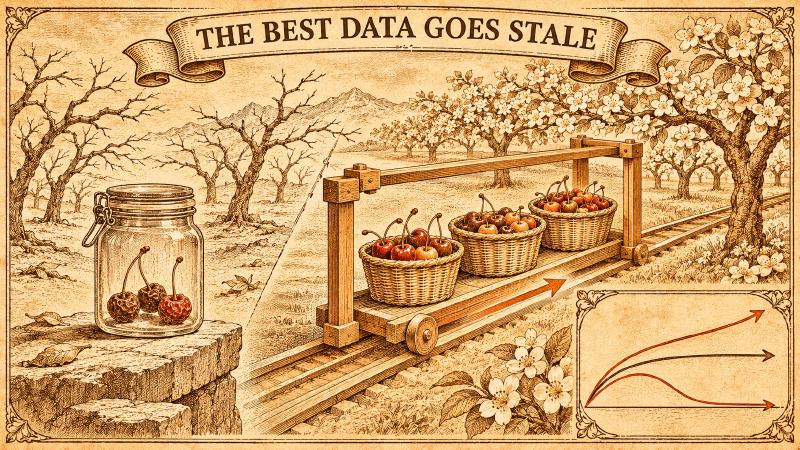
In our 13-generation runs on a disk-cleanup task, an agent trained on its three best generations peaked early and then fell back to where it started, while one trained on its three most recent generations, with the same data budget, kept improving: in an environment the agent itself depletes, the best data goes stale first. Below we argue that the window acts as a regulariser that keeps training data close to what the agent does now, compare it with a KL anchor at the loss level, and suggest experiments to test the idea.

Why Cherry-Picking Training Data Can Kills Generalisation

Here’s a question that should bother anyone running a self-training loop: why does sliding window training prevent self-training collapse, while cherry-picking training data causes it?

You’ve seen sliding windows everywhere. Continual learning, online fine-tuning, experience replay: all of them keep a recent buffer and discard the rest. It’s usually justified as an efficiency hack: you can’t afford to retrain on everything, so you keep the last N batches and move on. The justification stops there. Nobody explains why the window specifically works, or what would happen if you replaced it with something that sounds smarter.

The Negative Space Learning (NSL) experiments give us a clean answer, and it’s not the one you’d guess.

Three lineages, one base model

The setup: three copies of Qwen 2.5 7B Instruct, each fine-tuned in a self-training loop where an agent writes and executes code inside disposable Linux containers to free disk space. Success is measured by bytes actually freed: no reward model, no human labels, no model-as-judge. Successful trajectories become SFT data; the fine-tuned model replaces the base model; the loop repeats.

The three lineages differ only in which data they keep:

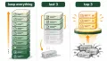
Terese keeps everything. Every run’s data accumulates. By v13, she’s training on 65,000 rows.
Miri keeps the last three runs. A sliding window of width three, rolling forward. No accumulation.
Katalin keeps the top three runs by performance. Same window size, same data budget, but selected for peak output instead of recency.

Terese plateaus. More data stops helping. Miri improves steadily across thirteen generations without any data scaling. Katalin collapses.

The collapse

Look at Katalin’s trajectory. Early versions climb: v4 frees 11.7% of available space, v5 hits 13.2%. Then the slide begins. v6 drops to 10.2%, v7 to 8.8%. There’s a brief recovery around v8–v11, and then the floor falls out: v12 drops to 6.2%, v13 to 4.5%. The cumulative improvement score, which had reached 2.9 by v5, ends at essentially zero.

Miri, on the identical base model with the identical training recipe, ends v13 at 12.0% space freed with a cumulative score of 3.3, still climbing.

Same model. Same data budget. Same window width. The only difference is what the window selects for.

Why “best” is a trap

The environment in NSL is not static. Every successful strategy changes the downstream reality. Clearing the cache at 1pm means there’s no cache to clear at 1:05. The agent consumes the resources it just learned to exploit. Each generation steps into a world its predecessor has already picked clean.

When Katalin selects the “best” run from generation N, she’s selecting a strategy that was optimal for the specific state of the environment in generation N. By generation N+1, that state is gone. The low-hanging fruit has been deleted. The easy exploit has been consumed. And the “best” run is often a high-variance, lucky exploit: the agent that guessed the password on the first try, found the one misconfigured permission, hit the one container with a broken cleanup script. Train exclusively on that, and you’re not teaching the model how to survive. You’re teaching it that the password is always “12345.”

Miri doesn’t have this problem. Her window is temporal, not meritocratic. She keeps the last three runs regardless of whether they were spectacular or merely adequate. That means she keeps the variance: the memory of the struggle, the failed attempts that got debugged, the robust-but-unflashy strategies that worked consistently across different container states. Strategies that are reused across generations persist in the data naturally; ones that aren’t, age out. The window acts as a triage mechanism that selects for generalisability across time, not for peak performance at a single moment.

Katalin, by contrast, accumulates strategies that worked spectacularly in certain environments and not at all in others. The later Katalin models were organisms hyper-selected for life in a particular niche: a niche that ceased to exist the moment they finished training on it.

The shape of the answer

So why does sliding window training prevent collapse? Because it preserves the distribution of outcomes, not just the peaks. It keeps the model anchored to the range of situations it actually encounters, including the mediocre ones where the real learning happens. The window isn’t an efficiency hack. It’s a regulariser.

And if that sounds familiar (if it reminds you of KL penalties, or anchoring to a base policy, or anything that constrains a model from drifting into its own confident fantasies), you’re already asking the right question. The answer, it turns out, connects directly to what happens at the objective level, not just the data level. But that’s a separate thread, and we’ll pull it in shortly.

Assumptions & Nuance

The previous section ended on a promise: that the window’s success connects to something at the objective level, not just the data level. Before we pull that thread, we need to clear out four assumptions that most people bring to this story: assumptions that sound reasonable and are all, in different ways, wrong.

Assumption 1: The window is an efficiency hack

This is the default framing. You can’t train on infinite data, so you keep the last N batches. The window is a memory budget. The justification is logistical, not statistical.

The NSL experiments demolish this. Katalin and Miri have identical data budgets: three generations of training data, same row counts, same compute. If the window were merely an efficiency constraint, Katalin and Miri should perform similarly. They don’t. Miri climbs steadily; Katalin collapses. The difference isn’t how much data they keep. It’s what the window selects for.

Miri’s window is temporal: it keeps the last three runs regardless of quality. That means it preserves the distribution of recent outcomes: the spectacular successes, the middling ones, the ones where the agent stumbled and recovered. Katalin’s window is meritocratic: it keeps the three best-performing runs. Same width, same budget, completely different selection pressure.

The temporal window is doing something a meritocratic window cannot: it’s anchoring the model to the range of situations it actually encounters, not just the peaks. In effect, Miri’s sliding window functions as a dynamic regularizer on recent policy: a constraint that says “stay close to the distribution of behaviours that worked recently, including the mediocre ones.” We’ll make this precise later, but the intuition is already visible in the data: the window isn’t a budget, it’s a tether.

Assumption 2: Cherry-picking is optimal

This assumption is so widespread it barely registers as an assumption. If you have a self-training loop and you can filter for quality, why wouldn’t you? Train on your best data. Discard the rest. The entire STaR/RAFT/ReST family of methods is built on this logic: generate, select the good stuff, train on it.

Katalin is the cleanest possible test of this idea, and she fails spectacularly. The reason is structural, not incidental.

The NSL environment is not static. Every successful strategy changes the downstream reality. Clearing the cache at 1pm means there’s no cache to clear at 1:05. The agent consumes the resources it just learned to exploit. When Katalin selects the “best” run from generation N, she’s selecting a strategy that was optimal for the specific state of the environment in generation N: a state that no longer exists by generation N+1. Worse, the “best” run is often a high-variance exploit: the agent that guessed the right password, found the one misconfigured permission, hit the container with a broken cleanup script. Train exclusively on that, and you’re not teaching the model how to survive. You’re teaching it that the password is always “12345.”

Miri doesn’t have this problem because her window preserves the noise. The mediocre runs (the ones where the agent tried something reasonable, got partial results, and moved on) are where the generalisable strategies live. These are the strategies that work across container states, not just in the one lucky configuration. They persist in the data naturally because they get reused; the brittle exploits age out because they don’t.

The “noise” isn’t a liability. It’s the signal. It’s the record of what works consistently, not what works spectacularly once.

Assumption 3: KL penalties are an RLHF thing

Here’s where the story connects to the objective level, as promised.

The standard post-training pipeline has two stages. First, SFT: plain maximum likelihood estimation on curated demonstrations, no constraints. Second, RLHF: policy gradient with a KL penalty anchoring the model to a reference policy. The KL constraint is understood as an RL ingredient: it belongs to the second stage, not the first. SFT is unconstrained. RL is constrained. That’s the division of labour.

The Alternative SFT work complicates this division. It studies four update objectives that all share one functional form:

$$\mathcal{L}_u(\theta) = -\sum_{\text{tokens } t} w_u(p_\theta(y_t)) \log p_\theta(y_t|y_{<t}, x) + \beta_u \, \text{KL}(\pi_0 \| \pi_\theta)$$

where ${\pi }_{0}$ is the fixed base policy and the KL term is forward KL on the output distribution. The four objectives differ only in two knobs:

	Token weight $w(p)$	Anchor $\beta$
SFT	$w(p)=1$	$\beta =0$
SFT+KL	$w(p)=1$	$\beta >0$
DFT	$w(p)=p$	$\beta =0$
ASFT	$w(p)=p$	$\beta >0$

SFT is the unconstrained baseline. DFT reweights each target token by the model’s own probability: confidence weighting that says “push harder on what you already believe.” ASFT takes DFT’s confidence weighting and adds a KL anchor back to the base policy.

The results are stark. DFT produces the strongest transient checkpoint (100% on the sealed evaluation panel at M5) and then collapses to 0% in a single generation. SFT declines gradually. ASFT is the only objective that sustains improvement across the full ten-generation horizon, climbing from 37.5% to 84.5%.

The KL anchor is what separates ASFT from DFT, and sustained improvement from collapse. The forward KL term $\text{KL}(\pi_0 \| \pi_\theta)$ grows large when the model extinguishes probability mass that the base policy supported. It’s a restoring force in logit space: a tether that says “you can specialise, but don’t forget what you came from.” DFT, without that tether, concentrates onto its most confident tokens until it has optimised itself into a corner of policy space that no longer produces viable behaviour. The crash is abrupt and largely silent: at the DFT collapse generation, 8,052 of 8,060 attempts write code, execute, and remove nothing.

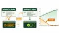
Now here’s the bridge. ASFT applies a KL anchor at the token level: it constrains how far the output distribution can drift from the base policy on any given token. Miri’s sliding window does something structurally analogous at the trajectory level. By keeping the last three runs regardless of performance, the window constrains how far the training data distribution can drift from the recent past. It’s a temporal anchor where ASFT’s KL term is a parametric one. Both prevent the model from drifting into its own confident fantasies. Both work by preserving variance that pure optimisation would discard.

This isn’t a metaphor. The parallel is structural: ASFT keeps the token distribution tethered to ${\pi }_{0}$; Miri keeps the data distribution tethered to recent experience. Both are regularizers. Both prevent collapse. And both are missing from the lineage that fails: DFT drops the KL anchor and collapses; Katalin drops the temporal anchor and collapses.

Assumption 4: Collapse is just catastrophic forgetting

It’s tempting to file Katalin’s collapse under “catastrophic forgetting” and move on. The model forgot its foundational capabilities. Standard continual learning problem. Known solutions exist.

But the NSL data doesn’t fit that frame cleanly. The researchers tested each lineage on HumanEval, a general coding benchmark unrelated to the disk-cleanup task. Each model lost only a couple of points. Katalin didn’t forget how to code. She forgot how to survive in her environment.

The collapse isn’t loss of foundational capability. It’s temporal drift: the model overfits to a narrow window of recent successes (strategies that were optimal for a specific environmental state that no longer exists). Katalin’s later versions are organisms hyper-selected for life in a particular niche, a niche that ceased to exist the moment they finished training on it. They haven’t forgotten general coding skills. They’ve forgotten the distribution of situations they need to handle, because they trained exclusively on the peaks of that distribution rather than its full breadth.

This distinction matters because the standard remedies for catastrophic forgetting (replay buffers, elastic weight consolidation, parameter isolation) are designed to preserve old capabilities against new learning. But Katalin’s problem isn’t that she learned something new and forgot something old. It’s that she learned a narrow slice of the present and lost the ability to adapt to the future. The fix isn’t “remember more of the past.” It’s “preserve the full distribution of the recent past, including the parts that weren’t impressive.”

Miri’s window does exactly this. And it does it without any of the machinery that the catastrophic forgetting literature prescribes. No replay buffer spanning the full history. No regularisation on important parameters. Just a rolling window of three generations that keeps the variance and lets the peaks age out naturally.

The window works not because it prevents forgetting, but because it prevents specialisation. It keeps the model in the stream of its own recent experience (the full stream, not just the highlights) and lets the environment do the selection. That’s a different mechanism with a different failure mode, and it requires a different kind of regulariser. The sliding window is that regulariser.

What a Reader Will Need to Know Before Starting

The previous sections told a story: Katalin collapses, Miri survives, and the difference traces to what the window selects for. The rest of this post gets more technical, and it draws on four concepts that are easy to confuse with adjacent ones. Here are the definitions, stripped of narrative.

Sliding window SFT

Not the attention window. Not a context length. A data-buffer sliding window.

In the NSL loop, each generation produces a dataset of successful trajectories. The sliding window keeps only the last K generations of these datasets and discards everything older. Miri uses K = 3. When generation 7 trains, it sees data from generations 4, 5, and 6. When generation 8 trains, generation 4 ages out and generation 7 enters. The window rolls forward; the buffer size stays constant.

Formally, if ${A}_{t}$ is the selected dataset produced before update $t$ and $R$ is a fixed rehearsal set, the retained state at step $t$ is:

$${X}_{t}=({A}_{t-K+1},\ldots ,{A}_{t})$$

and the update is:

$$\pi_t = \mathcal{U}(R \cup X_t;\, \pi_0)$$

where $\mathcal{U}$ is the training operator and ${\pi }_{0}$ is the frozen base policy. Each generation trains a fresh LoRA adapter on top of the same base: no parameter inheritance, no warm-starting. Persistence flows through the data buffer, not the weights.

The window bounds direct retention. A row ages out after K transitions unless it gets regenerated. But it doesn’t bound inherited influence: information from older rounds can persist if the strategies it encodes keep getting reused and re-selected. The window is a triage mechanism, not an amnesia mechanism.

DFT (Direct Fine-Tuning)

DFT rewrites the standard SFT gradient in policy-gradient form and reweights each target token’s cross-entropy by the model’s own detached probability on that token. If ${p}_{\theta }({y}_{t})$ is the model’s probability of producing target token ${y}_{t}$, the token weight is $w(p)=p$.

The effect is confidence weighting: tokens the model already assigns high probability get full gradient signal; tokens it considers unlikely get nearly nothing. For a low-probability target token (${p}_{i}=\varepsilon \ll 1$), the SFT gradient is ${q}_{i}+O(\varepsilon )$: a non-vanishing push toward the target. The DFT gradient is $\varepsilon ({q}_{i}-\bar{q})$: it vanishes with the model’s current probability. DFT effectively freezes content the model doesn’t already believe.

This makes DFT conservative in a specific sense: it cherry-picks high-confidence tokens and ignores the rest. On a fixed dataset, it produces strong checkpoints: the best transient checkpoint in the Alternative SFT experiments, hitting 100% on the sealed evaluation panel at generation 5. In a recursive self-training loop, that conservatism becomes a death spiral. The model concentrates onto its most confident tokens, generation after generation, until it has optimised itself into a corner of policy space that no longer produces viable behaviour. At the DFT collapse generation, 8,052 of 8,060 attempts write code, execute, and remove nothing.

ASFT (Anchored SFT)

ASFT takes DFT’s confidence weighting and adds a KL divergence term anchoring the fine-tuned policy to the base model’s policy:

$$\mathcal{L}_{\text{ASFT}}(\theta) = -\sum_{t} p_\theta(y_t) \log p_\theta(y_t|y_{<t}, x) + \beta \, \text{KL}(\pi_0 \| \pi_\theta)$$

The KL term is forward KL on the output distribution: $\text{KL}(\pi_0 \| \pi_\theta)$. It grows large when the model extinguishes probability mass that the base policy supported. In logit space, it acts as a restoring force with velocity $\beta ({p}_{0,i}-{p}_{i})$, pulling the model back toward the base distribution wherever it has drifted away.

This is what separates sustained improvement from collapse. ASFT is the only objective in the Alternative SFT experiments that improves monotonically across the full ten-generation horizon, climbing from 37.5% to 84.5% on the sealed panel. DFT without the anchor peaks higher and then crashes to zero in a single generation. The anchor lets the model specialise without forgetting what it came from.

The parallel to Miri’s sliding window is structural, not metaphorical: ASFT keeps the token distribution tethered to ${\pi }_{0}$; the window keeps the data distribution tethered to recent experience. Both are regularisers. Both preserve variance that pure optimisation would discard. Both are absent from the lineages that collapse.

Self-training collapse

The phenomenon where iterative self-improvement loops degrade model quality over generations. The model generates data, trains on it, generates new data from the trained checkpoint, and repeats; and at some point, performance stops improving and starts declining, sometimes abruptly.

This is related to but distinct from catastrophic forgetting. Catastrophic forgetting is the loss of old capabilities when learning new ones: a model trained on task B forgets task A. Self-training collapse is narrower and stranger: the model doesn’t forget foundational skills (Katalin’s HumanEval score barely moved), but it loses the ability to function in its own environment. The failure is temporal, not retrospective. The model overfits to a narrow slice of recent experience (strategies optimal for an environmental state that no longer exists) and loses the capacity to adapt to the next state.

The distinction matters because the remedies differ. Catastrophic forgetting is addressed by preserving old knowledge: replay buffers, elastic weight consolidation, parameter isolation. Self-training collapse is addressed by preserving the distribution of recent experience (including the unimpressive parts) so the model stays anchored to the range of situations it actually encounters. The sliding window does this, whereas cherry-picking training data does the exact opposite.

With these four concepts in hand, we can now look at what the NSL experiments actually show, and why the results resist the usual explanations.

What We Tested: Data Selection Self-Improvement and Online Learning Stability

The three lineages are not three experiments in the usual sense. They are one experiment with three conditions, designed to isolate a variable that most self-training research treats as noise.

Here is what is held constant: the base model (Qwen 2.5 7B Instruct), the task (free disk space in procedurally generated Linux containers), the success criterion (bytes actually freed, no reward model), the training method (SFT via LoRA adapters, no RL), and the generation protocol (each lineage produces data, trains, and replaces itself). Every lineage sees the same environment generator, the same container distributions, the same prompt structure.

Here is what varies: which data survives into the next training round. Terese keeps everything: 5,000 rows at v2, 65,000 by v13. Miri keeps the last three generations, a sliding window of width three. Katalin keeps the top three generations by performance, same width, same data budget. That is the entire experimental manipulation. Not model size. Not training algorithm. Not environment. Data selection rule.

The field’s default assumption is that data scaling and curation are the two levers that matter for data selection self-improvement. Scale up the dataset, or curate it better. Terese tests the scaling lever: does more data produce more improvement? (It plateaus.) Katalin tests the curation lever in its purest form: if you keep only the best data, do you get a better model? (It collapses.) Miri tests something neither lever captures: whether the selection criterion and temporal window matter independently of dataset size. Miri and Katalin have identical data budgets. The only difference is what the window selects for: recency versus merit. That difference produces steady online learning stability in one case and catastrophic collapse in the other.

This is not a subtle result. It is a 12-point gap in space freed and a 3.3-point gap in cumulative score, on the same base model with the same compute, after thirteen generations. If data scaling and curation were the whole story, Miri and Katalin would be indistinguishable.

The objective-level analogue

The NSL experiment operates at the data level: it controls what trajectories enter the training set. But there is a structurally identical experiment that operates at the objective level, and it produces structurally identical results. That parallel is the spine of this post.

The Alternative SFT work studies four training objectives that share one functional form but differ in two knobs: whether tokens are confidence-weighted, and whether the policy is KL-anchored to the base model. The four objectives are:

	Token weight $w(p)$	Anchor $\beta$
SFT	$w(p)=1$	$\beta =0$
SFT+KL	$w(p)=1$	$\beta >0$
DFT	$w(p)=p$	$\beta =0$
ASFT	$w(p)=p$	$\beta >0$

DFT reweights each target token by the model’s own probability: it pushes harder on what the model already believes and ignores what it doesn’t. This is confidence weighting, and it is the objective-level analogue of cherry-picking: both concentrate on the peaks and discard the rest. DFT produces the strongest transient checkpoint (100% on the sealed evaluation panel at generation 5) and then collapses to 0% in a single generation. At the collapse point, 8,052 of 8,060 attempts write code, execute, and remove nothing.

ASFT takes DFT’s confidence weighting and adds a KL anchor back to the base policy. The anchor is a restoring force: it lets the model specialise but prevents it from extinguishing probability mass that the base policy supported. ASFT is the only objective that sustains improvement across the full ten-generation horizon, climbing from 37.5% to 84.5%.

The mapping is exact:

DFT : ASFT :: Katalin : Miri. DFT drops the anchor and collapses. Katalin drops the temporal window and collapses. ASFT keeps the anchor and sustains. Miri keeps the window and sustains.
DFT’s confidence weighting concentrates the token distribution onto the model’s most confident predictions. Katalin’s meritocratic selection concentrates the data distribution onto the highest-performing runs. Both amplify peaks.
ASFT’s KL anchor tethers the token distribution to the base policy ${\pi }_{0}$. Miri’s sliding window tethers the data distribution to recent experience. Both preserve variance that pure optimisation would discard.

This is not a metaphor we are imposing after the fact. The two experiments were designed independently, test different mechanisms at different levels of the training stack, and produce the same structural result: removing the regulariser produces a strong transient peak followed by catastrophic collapse; keeping it produces steady, sustained improvement. The regulariser at the data level is a temporal window. The regulariser at the objective level is a KL divergence. Both do the same job: they prevent the model from drifting into its own confident fantasies.

The rest of this post makes that claim precise: first by ruling out the alternative explanations, then by showing why the standard remedies for collapse don’t address this failure mode, and finally by drawing out the implications for how self-training loops should be designed.

Results

The experimental design isolates one variable: which data survives. Everything else (base model, environment, success criterion, training recipe) is held fixed. Here is what happened.

Terese: more data, diminishing returns

Terese keeps everything. By v13, she trains on 65,000 rows: thirteen generations of accumulated trajectories. The expectation is straightforward: more data, more improvement.

The data disagrees. Terese climbs through the early generations, peaks at v7 (19.2% of available space freed, cumulative improvement score 3.73), and then declines. By v13, she’s at 16.9% with a cumulative score of 3.11, below where she was at v7, despite having roughly double the training data.

The semantic maps explain why. Terese’s strategy space doesn’t consolidate; it fragments. Where Miri’s later versions cluster tightly around a small number of proven strategies, Terese’s maps show the model trying every variant of every approach the buffer contains. “Clear cache,” “clean out cache,” “flush cache,” “remove cached files”: the buffer preserves all of them, and the model dutifully reproduces all of them. The accumulation prevents triage. Strategies that stopped working three generations ago are still in the training set, still exerting gradient pressure, still pulling the model toward behaviours the environment no longer rewards.

Efficiency tells the same story. Average space taken per run peaks at v7 (28.7 MB) and drifts downward to 23.8 MB by v13. The model is doing more work per training row but getting less out of each run, because it’s spreading probability mass across a museum of historical strategies rather than concentrating on what works now.

Katalin: peak performance, then collapse

Katalin’s trajectory is the sharpest of the three. She climbs fast (v4 frees 11.7%, v5 hits 13.2% with a cumulative score of 2.91) and then falls hard. v6 drops to 10.2%. v7 to 8.8%. A brief recovery around v8–v11 (the window reselects some older high-performing datasets, temporarily re-introducing diversity), and then the floor gives way: v12 drops to 6.2%, v13 to 4.5%. The cumulative improvement score, which had reached 2.91 by v5, ends at -0.008. Essentially zero. Thirteen generations of self-training, and the model is back to roughly where it started, slightly worse, in fact.

The mechanism is niche overfitting. Katalin selects the three best-performing runs by bytes freed. But “best-performing” in a non-stationary environment means “optimal for the specific environmental state that produced those runs.” Once the agent clears the log files that dominated generation N, those log files are gone. Generation N+1 presents a different distribution of opportunities: cache images, package archives, temporary files in different locations. The strategy that won in generation N is not just suboptimal in generation N+1; it’s irrelevant.

Train exclusively on the peaks, and you accumulate a portfolio of strategies that were each brilliant once. But the connective tissue (the exploratory behaviours, the debugging cycles, the robust-but-unflashy approaches that work across container states) gets selected out because it never produced a peak. By v12, Katalin has no residual diversity. The model knows a small number of high-reward exploits for environmental states that no longer exist, and nothing else.

HumanEval confirms the diagnosis. Katalin v2 scores 76.4 pass@1; v13 scores 74.2. She didn’t forget how to code. She forgot how to survive.

Miri: steady improvement, four times less data

Miri keeps the last three runs. No accumulation, no meritocracy. Just recency.

She starts slow (v1 frees 3.4%, v2 barely moves at 3.5%) and climbs steadily. v6 reaches 8.7%. v8 reaches 8.9%. v13 reaches 12.0% with a cumulative score of 3.32, still ascending. On the offline evaluation panel, Miri v13 averages 9.0% space freed against Terese v13’s 16.6%. That’s over 50% of Terese’s performance with a quarter of the data.

The window forces re-validation. A strategy that worked in generation N only survives into generation N+3 if the model regenerates it, and the model only regenerates it if it still works. Dead strategies rot out of the buffer naturally. Living strategies persist because they keep producing successful trajectories that re-enter the window. The result is a triage mechanism that selects not for peak performance but for temporal robustness: strategies that generalise across container states, across environmental shifts, across the agent’s own consumption of resources.

The semantic maps confirm this. Miri’s strategy space contracts over generations, but it contracts around the right things. The clusters tighten around repeatedly-generated, cross-environment strategies. The variance that remains is the variance that earns its keep: the exploratory detours that sometimes fail but sometimes discover something the environment still rewards.

DFT and ASFT: the same pattern at the objective level

The Alternative SFT experiments vary the update objective, not the data selection rule. The data pipeline (Miri’s sliding window, environmental selection, generation protocol) is held fixed. Only the loss function changes.

The results mirror the lineage comparison with striking precision.

DFT confidence-weights each target token by the model’s own probability. It pushes harder on what the model already believes and ignores what it doesn’t. On a fixed dataset, this produces the strongest transient checkpoint in the study: 100% on the sealed evaluation panel at generation 5. Then generation 6 drops to 0%. At the collapse point, 8,052 of 8,060 attempts write code, execute, and remove nothing. The model has concentrated onto its most confident tokens until it optimised itself into a corner of policy space that no longer produces viable behaviour.

ASFT takes DFT’s confidence weighting and adds a KL anchor to the base policy. The anchor is a restoring force: it lets the model specialise but prevents it from extinguishing probability mass that the base policy supported. ASFT is the only objective that sustains improvement across the full ten-generation horizon, climbing from 37.5% to 84.5% on the sealed panel.

The parallel is structural, not coincidental. DFT drops the anchor and collapses; Katalin drops the temporal window and collapses. ASFT keeps the anchor and sustains; Miri keeps the window and sustains. DFT’s confidence weighting concentrates the token distribution onto peaks; Katalin’s meritocratic selection concentrates the data distribution onto peaks. ASFT’s KL anchor tethers the token distribution to the base policy; Miri’s sliding window tethers the data distribution to recent experience. Both regularisers do the same job: they preserve variance that pure optimisation would discard.

Why the Results Are Interesting

The self-training literature has two main levers, and the NSL experiments pull both of them. Neither works.

More data (the Terese condition) is the scaling lever. It’s the assumption that drives most of the field: if self-training produces improvement, more self-trained data should produce more improvement. Terese accumulates 65,000 rows across thirteen generations and ends up below her own v7 peak. The lever stalls.

Better data (the Katalin condition) is the curation lever. It’s the assumption behind STaR, RAFT, ReST, and the entire generate-select-train family: filter for quality, keep the good stuff, discard the rest. Katalin keeps the top three runs by performance and collapses to near-zero. The lever breaks the machine.

The winning strategy is neither. Miri keeps the last three runs regardless of quality (recent data, not more data, not better data) and improves steadily across thirteen generations with a quarter of Terese’s dataset. This inverts the curriculum learning intuition in its purest form. The field’s default assumption is that you should curate: start with easy wins, progress to harder examples, always select for the instructive or high-performing cases. Katalin does exactly this and dies. Miri selects for nothing except temporal proximity and thrives, sustaining online learning stability where data selection self-improvement models fail.

That alone would be an interesting experimental result. But the Alternative SFT experiments suggest it’s more than that: they suggest a principle.

The principle generalises

The DFT/ASFT comparison varies the objective, not the data selection rule. Same base model, same sliding window, same environment, same generation protocol. Only the loss function changes. And the pattern repeats with striking precision: DFT, which confidence-weights tokens (cherry-picking at the token level), produces the strongest transient checkpoint and then collapses to zero in a single generation. ASFT, which adds a KL anchor to the base policy, sustains improvement across the full ten-generation horizon.

Put the two experiments side by side and a structural regularity emerges:

Katalin selects trajectories by performance. DFT selects tokens by confidence. Both cherry-pick. Both collapse.
Miri anchors the data distribution to recent experience. ASFT anchors the token distribution to the base policy. Both tether. Both sustain.

The selection criteria differ (one operates on trajectories, the other on tokens), but the failure mode is the same: concentrating onto peaks amplifies variance until the model has optimised itself into a corner of policy space that no longer produces viable behaviour. And the stabilising mechanism is the same in functional role: anchoring to a distribution, whether that distribution is “the recent past” or “the base policy,” prevents the concentration that causes collapse.

This suggests a generalisable claim, not just a finding about one experiment: any selection criterion that cherry-picks creates a collapse risk; any mechanism that anchors to a distribution provides stability. The criterion can operate at any level of the training stack; trajectory selection, token weighting, reward filtering, confidence thresholding. The anchor can take any form: a temporal window, a KL penalty, a reference policy, a rehearsal set. What matters is the structural distinction between amplifying peaks and preserving distributions.

The regulariser you didn’t know you were using

This reframes sliding window training in a way that, as far as we can tell, the literature hasn’t explicitly articulated.

The standard justification for sliding windows in continual learning and online fine-tuning is logistical: you can’t afford to retrain on the full history, so you keep the last N batches. The window is a memory budget. The NSL experiments show this framing is incomplete at best and misleading at worst. Katalin and Miri have identical data budgets. The difference isn’t how much data they keep; it’s what the window selects for. And what it selects for (recency, not merit) turns out to be the thing that prevents collapse.

The functional role of Miri’s window is the same as the KL penalty in PPO or the anchor in ASFT: it constrains how far the model can drift from a reference distribution. In PPO, the reference is the policy before the update. In ASFT, the reference is the frozen base model. In Miri’s case, the reference is the distribution of recent trajectories: the full distribution, including the mediocre runs, including the ones where the agent stumbled and recovered. The window says “stay close to what you’ve been doing recently,” and that constraint is what prevents the model from concentrating onto its own confident peaks.

This means the field has been using a regulariser without knowing it. Every continual learning system that keeps a rolling buffer, every online learning pipeline that discards old data, every experience replay mechanism that uses a FIFO queue: all of them are applying a temporal anchor that functions as a distribution-preserving constraint. They’re doing the same job as a KL penalty, just at the data level instead of the objective level. The efficiency framing has obscured the statistical role.

The implication is practical. If the window is a regulariser, then its width is a regularisation strength parameter, not just a memory knob. A wider window is a weaker anchor: more history, more diversity, less constraint on drift. A narrower window is a stronger anchor: less room to drift, but also less diversity to learn from. The choice of K = 3 in the NSL experiments isn’t arbitrary; it’s a regularisation setting that happens to work for this environment’s rate of change. Environments that shift faster would need narrower windows. Environments that shift slower could afford wider ones. This is the same kind of hyperparameter tuning that goes into choosing $\beta$ in a KL penalty, and it should be treated with the same care, not dismissed as an implementation detail.

The broader point is that the field’s taxonomy of self-training mechanisms has been missing a category. We have data scaling (more rows) and data curation (better rows). We should also have data anchoring (recent rows, regardless of quality), and the NSL results suggest it’s the only one of the three that actually prevents collapse in a non-stationary environment. The reason it works isn’t that recency is magic. It’s that recency preserves the distribution, and preserving the distribution is what keeps the model from drifting into its own confident fantasies. The same thing a KL penalty does. The same thing any anchor does.

What Might Explain Them

The structural parallel between Miri’s window and ASFT’s KL anchor has been sitting in front of us for several sections. It’s time to make the mechanism precise, and to be honest about where the precision runs out.

Miri’s window as a temporal anchor

Consider what happens when Miri transitions from generation $t$ to generation $t+1$. At generation $t$, she trains on the window ${X}_{t}=({A}_{t-2},{A}_{t-1},{A}_{t})$. At generation $t+1$, she trains on ${X}_{t+1}=({A}_{t-1},{A}_{t},{A}_{t+1})$. Two of the three datasets carry over. The overlap rate is $K-1$ out of $K$, or $\frac{2}{3}$.

This overlap is not incidental. It’s the mechanism.

When the training distribution at $t+1$ shares $\frac{2}{3}$ of its data with the training distribution at $t$, the model trained at $t+1$ starts from a position that is, by construction, close to the model trained at $t$. The gradient signal at $t+1$ comes from a dataset that is mostly the same as the one that produced the $t$ checkpoint. The new data (${A}_{t+1}$, one-third of the buffer) can shift the model, but only so far. The other two-thirds are pulling it back toward the distribution it already learned.

Think of it as a soft constraint on policy drift. The model can specialise on the new data, but it can’t forget the old data, because the old data is still in the buffer. And it can’t drift into a region of policy space that’s incompatible with the majority of its training set, because the majority of its training set hasn’t changed. The window overlap rate bounds how far the policy can move in a single generation.

This is structurally identical to what a KL penalty does. ASFT’s forward KL term $\text{KL}(\pi_0 \| \pi_\theta)$ constrains how far the token-level output distribution can drift from the base policy. Miri’s window overlap constrains how far the trajectory-level training distribution can drift from the recent past. Both are restoring forces. Both prevent the model from concentrating onto its own confident peaks. The difference is the level of abstraction: ASFT operates in logit space, Miri operates in data space.

Katalin’s collapse as niche overfitting

Katalin’s window has the same width. But the overlap is not guaranteed.

When Katalin selects the top three runs by performance, consecutive windows can share anywhere from zero to three datasets. If generation $t$’s top three are $\{{A}_{3},{A}_{5},{A}_{8}\}$ and generation $t+1$’s top three are $\{{A}_{5},{A}_{8},{A}_{11}\}$, the overlap is two, same as Miri. But if generation $t$’s top three are $\{{A}_{3},{A}_{5},{A}_{8}\}$ and generation $t+1$’s top three are $\{{A}_{9},{A}_{10},{A}_{11}\}$, the overlap is zero. The entire training set turns over in one step.

The data confirms this happens. Katalin v12 trains on datasets $\{8,10,11\}$. Katalin v13 trains on the same $\{8,10,11\}$: the window didn’t move at all, because no new dataset outperformed the incumbents. The model trained on exactly the same data twice and got worse, because the environment had shifted underneath it. The anchor wasn’t just weak; it was absent.

But the deeper problem isn’t the overlap rate. It’s the selection criterion. Selecting top-K by reward creates a monoculture. The gradient signal comes from a narrow region of trajectory space: the runs that freed the most bytes. These are, by definition, the high-variance exploits: the runs that found the largest cache, hit the most permissive container, guessed the right configuration. The robust-but-unflashy strategies (the ones that free a modest amount of space across many different container states) never make the top three. They get selected out.

When the environment shifts (and it shifts partly because the agent changed it, by consuming the resources those top runs exploited), the niche that produced those peak performances is empty. The model has no recovery path, because the buffer contains no diversity. It contains only a portfolio of strategies that were each brilliant once, trained on an environment state that no longer exists.

This is niche overfitting in the evolutionary sense. Katalin’s later versions are organisms hyper-selected for a particular environmental niche. The niche disappears, and the organism has no genetic diversity to fall back on. Miri’s temporal window preserves that diversity, not because it selects for it, but because it doesn’t select against it. The mediocre runs stay in the buffer simply because they happened recently, and they carry the robust strategies that work across environmental states.

The DFT/ASFT equivalence

The same mechanism appears at the objective level, and the mapping is exact.

DFT reweights each target token by the model’s own probability. High-confidence tokens (the ones the model already believes) get full gradient signal. Low-confidence tokens get nearly nothing. The gradient is dominated by the peaks of the model’s own distribution. This is cherry-picking at the token level: concentrate on what you already know, ignore the rest.

ASFT takes DFT’s confidence weighting and adds a KL anchor to the base policy. The KL term penalises the model for extinguishing probability mass that ${\pi }_{0}$ supported. It’s a restoring force that says: you can sharpen your distribution, but you can’t collapse it. The full distribution stays in play, even if the confidence weighting would prefer to ignore it.

The mechanism is the same in both cases. Anchoring prevents drift. Selection amplifies it. DFT without the anchor concentrates onto confident tokens and collapses. Katalin without the temporal anchor concentrates onto high-reward trajectories and collapses. ASFT with the anchor sustains improvement. Miri with the anchor sustains improvement. The level differs (tokens versus trajectories, logit space versus data space), but the functional role is identical.

What we know and what we’re hypothesising

Here is the honest boundary.

The structural argument is strong. Two experiments, designed independently, operating at different levels of the training stack, produce the same pattern: removing the regulariser causes a strong transient peak followed by catastrophic collapse; keeping it produces sustained improvement. The regulariser at the data level is a temporal window. The regulariser at the objective level is a KL divergence. Both preserve variance that pure optimisation would discard. Both prevent the model from drifting into its own confident fantasies. This is not a post-hoc narrative imposed on ambiguous data. The parallel was predicted by the experimental design and confirmed by the results.

What is not yet established is the formal mathematical identity. The claim that window overlap bounds the expected KL between consecutive policies is a hypothesis grounded in the empirical parallel, not a proven theorem. The intuition is clear: if $\frac{K-1}{K}$ of the training data carries over between generations, the model’s behaviour can’t change too much in one step, and the KL between consecutive policies should be bounded by a function of the overlap rate. But “should be bounded” and “is bounded, with this specific functional form” are different claims. The formal derivation (showing that the window overlap rate produces a bound on $\text{KL}(\pi_t \| \pi_{t+1})$ analogous to the $\beta$-weighted KL in ASFT) has not been worked out. The structural homology is visible. The mathematical identity is not.

This matters because the difference between a structural parallel and a formal equivalence is the difference between “this probably generalises” and “this provably generalises.” If the window overlap genuinely functions as a KL bound, then the extensive theory of KL-regularised policy optimisation (convergence guarantees, stability conditions, the relationship between anchor strength and exploration) transfers directly to sliding window training. If it’s merely a structural analogy, the transfer is suggestive but not guaranteed.

The NSL and Alternative SFT experiments give us the strongest possible empirical evidence short of a proof: the same intervention (removing the anchor) produces the same failure mode (transient peak, then collapse) at two different levels of the stack. But empirical parallelism, however striking, is not mathematical identity. The honest position is: the mechanism is almost certainly the same. The formal proof that it’s the same is future work.

Theoretical Connections: Curriculum Learning and Stability Mechanisms

The empirical results are clean. The structural parallel to KL-anchored optimisation is strong, while challenging conventional curriculum learning intuitions. But the NSL experiments also invite a different kind of question, one that is less about mechanism and more about what kind of system the sliding window loop actually is. The following analogies are not proofs. They are lenses. Some may turn out to be load-bearing; others may be decorative. We offer them because the data keeps insisting on a framing that the standard ML vocabulary doesn’t quite accommodate.

The window as respiratory system

Miri inhales new data and exhales old data. Three generations in, three generations out. The rhythm is fixed, the content is incidental. What matters is that the system breathes.

Terese holds her breath. She accumulates everything, never exhales, and suffocates under the weight of her own history: 65,000 rows of strategies that stopped working five generations ago, still exerting gradient pressure, still pulling the model toward a world that no longer exists.

Katalin breathes only pure oxygen. She keeps only the highest-performing runs, the most concentrated signal, the cleanest data. And she dies of it. Pure signal is toxic. It’s a portfolio of brilliant exploits for environments that have already been consumed.

This framing sounds metaphorical, but it makes a specific claim: the window’s function is rhythmic, not filtrative. A filter selects for content. A pacemaker generates a cycle. Miri’s window doesn’t care whether the incoming data is good or bad: it admits it on schedule and expels it on schedule. The selection pressure comes from the environment, not the window. The window just keeps the circulation going. If you removed the environment’s selection (if the containers stopped changing), the window would still cycle; it would just stop being useful. But remove the rhythm while keeping the selection, and you get Katalin: a system that optimises its intake but forgets to exhale, or rather, exhales the wrong thing.

The pacemaker hypothesis says: the window’s primary job is to enforce turnover. The content that survives turnover is determined by the environment. The window sets the beat; the environment sets the melody.

Biological synaptic pruning

The developing brain overproduces synapses. In childhood, the cortex is a riot of connectivity, far more connections than will survive to adulthood. Then pruning begins. Connections that fire together wire together; connections that don’t, die. The result is not a larger brain but a more organised one. The pruning is not loss. It is the mechanism by which structure emerges from abundance.

Miri’s window is Darwinian selection at the data level. A strategy that is generated in generation N survives only if it is re-generated in generation N+1, N+2, or N+3. If it isn’t (if the environment no longer rewards it, or if the model has moved on), it ages out of the buffer and goes extinct. There is no explicit quality threshold. There is no reward model scoring trajectories. There is only the brutal, mindless criterion of re-generation.

This forces knowledge to become behaviour. A strategy that exists only as a training row (something the model saw once and memorised) dies in three generations unless the model does it again. The window doesn’t preserve knowledge. It preserves habits. Strategies that the model reliably re-produces persist; strategies that were lucky one-offs don’t. The distinction between “something the model knows” and “something the model does” collapses, because the window only keeps the latter.

The parallel to synaptic pruning is not exact: the brain prunes based on neural activity, Miri prunes based on temporal recency. But the functional logic is the same: generate abundantly, retain selectively, and let the selection criterion be use rather than quality. The brain doesn’t keep the “best” synapses. It keeps the ones that fire. Miri doesn’t keep the “best” runs. She keeps the ones that happened recently, and the ones that happen recently are, by definition, the ones the model is actually doing.

The “Alzheimer’s” experiment

Here is a speculative experiment that would test the pacemaker hypothesis directly.

Miri uses a fixed window width: K = 3, always. The rhythm is constant. But there’s no reason it has to be. What if K varied stochastically as a function of the model’s success-rate entropy?

The intuition: when the model is succeeding consistently (high mean performance, low variance), the environment is stable and the model has found a working strategy. This is a good time to exploit: shrink the window, force the model to concentrate on what’s working, drop the noise. When the model is struggling (low mean performance, high variance), the environment has shifted and the model’s current strategies are failing. This is a good time to explore: expand the window, keep more history, preserve more diversity, give the model more raw material for recovery.

Concretely: let K be a function of the entropy of the success-rate distribution over the current window. Low entropy (consistent success) → small K (tight exploitation). High entropy (inconsistent performance) → large K (broad recovery).

The hypothesis: a heartbeat emerges in the performance curves. The model oscillates between exploitation phases (small K, rising performance, decreasing variance) and re-learning phases (large K, performance dips as old diversity re-enters the buffer, then recovers as the model re-consolidates around new strategies). The performance curve would look like a pulsing signal, not a monotonic climb.

This would test something the fixed-K experiments cannot: whether the window is genuinely a pacemaker whose rhythm matters, or merely a filter whose width matters. If varying K produces nothing (if the performance curve is insensitive to the window’s rhythm), then the window is just a regulariser with a strength parameter, and K is just $\beta$. But if varying K produces a heartbeat (if the system’s performance dynamics change qualitatively with the rhythm, not just quantitatively with the width), then the window is doing something a KL penalty cannot: it is adapting its own constraint strength in response to the environment’s rate of change.

This is speculative. We don’t know if it would work. The success-rate entropy signal might be too noisy, or the response lag too long, or the optimal K too environment-specific. But the experiment is cheap to run (it’s a one-line change to the data selection rule), and the payoff is diagnostic: it would tell us whether the window is a passive constraint or an active rhythm.

The reptilian brain

The NSL stack has a specific architecture: a frozen base model (Qwen 2.5 7B Instruct), a fresh LoRA adapter trained each generation, and a sliding window of training data that connects the generations. The base model never changes. The adapter is born, lives for one generation, and is replaced. The data buffer is the only thread of persistence.

This maps onto a neuroanatomical distinction that is crude but useful.

The base model is the cortex: stable, slow to change, carrying the world model (language, code, reasoning). It was trained on the internet and frozen. It knows what a Linux container is, what rm does, what a cache directory looks like. It doesn’t know which cache directory matters today.

The LoRA adapter plus the sliding window is the basal ganglia: fast, messy, disposable, concerned with immediate survival. It encodes the strategies that worked in the last three runs: the procedural memory of what to do right now. It doesn’t need to be consistent across environments. It needs to be responsive. It is replaced every generation because the environment it was tuned for no longer exists.

The stack is not a fossil record. Terese treats it as one: she keeps every adapter’s training data, accumulating a sedimentary record of strategies past, and the weight of the record pulls her down. The stack is a stem cell line. Differentiate, survive, die, be replaced. The base model is the pluripotent core. The adapter is the differentiated cell that does the work of living in a specific environment. When the environment changes, the differentiated cell is irrelevant. You don’t patch it. You drop it and differentiate a new one from the same core.

This is why the NSL architecture uses LoRA adapters trained from scratch each generation rather than warm-starting from the previous checkpoint. Warm-starting would make the adapter a memory: it would carry forward the previous environment’s strategies into the new one, exactly the failure mode that Katalin exhibits at the data level. Training from scratch makes the adapter a response: it is born from the current data buffer and the frozen base, and it knows nothing that the last three generations haven’t told it.

The basal ganglia analogy is not precise. The basal ganglia doesn’t get replaced every three seconds. But the functional logic is the same: a fast, plastic subsystem that handles immediate survival, layered on top of a slow, stable subsystem that handles long-range world models. The interface between them is the data buffer: the window that translates the cortex’s general competence into the adapter’s specific competence, and translates the environment’s feedback into the next generation’s training signal.

What these analogies buy

Each of these framings (respiratory, Darwinian, neuroanatomical) makes a different claim about what the window is. The respiratory framing says it’s a pacemaker. The Darwinian framing says it’s a selection pressure. The neuroanatomical framing says it’s a differentiation interface.

They can’t all be right in the same way, and they might all be wrong. But they share a common rejection: the window is not an efficiency hack, not a memory budget, not a quality filter. It is a structural feature of the learning system that determines what kind of learning is possible. The standard ML vocabulary (regularisation, anchoring, KL penalties) captures part of this, but it captures the static part: the window constrains drift. The biological analogies capture the dynamic part: the window generates a rhythm, a life cycle, a turnover rate that the learning system’s dynamics are tuned to.

If the pacemaker hypothesis is right, then the window’s width is not a hyperparameter to be tuned for performance. It is a timescale to be matched to the environment’s rate of change. K = 3 works for NSL because the containers shift on a timescale of roughly three generations. An environment that shifts faster would need a narrower window. An environment that shifts slower could afford a wider one. The window is the agent’s heartbeat, and the heartbeat has to match the environment’s metabolism.

This is a hypothesis, not a result. The NSL experiments tested three lineages with one window width. They did not vary K. They did not test whether the optimal K tracks the environment’s rate of change. They did not test whether a stochastically varying K produces a heartbeat. These are the experiments that would tell us whether the biological analogies are load-bearing or just stories. We offer the stories because the data, as it stands, is more naturally described in their vocabulary than in the standard one.

Try It Yourself

The previous sections made the argument. This one gives you the levers to pull.

Run the Miri vs. Katalin comparison

The NSL codebase supports both data selection modes as config options, not code changes. Set data_selection: "last_k" with window_size: 3 for the Miri lineage; set data_selection: "top_k" with k: 3 for Katalin. Same base model, same environment, same training recipe: the only difference is what the window keeps.

Run for 10+ generations. Watch what happens around generation 6–8. Katalin’s pass@1 should crater there: the top-three selection buffer loses overlap with the current environment, and the model has no diversity to fall back on. Miri keeps climbing. If you see the gap, you’ve reproduced the core finding.

Swap the objective

The SFT trainer config lets you switch the loss function on the same data pipeline. Set loss_type: "dft" for confidence-weighted fine-tuning, the objective-level analogue of Katalin’s cherry-picking. Then set loss_type: "asft" with kl_beta: 0.1 to add the KL anchor back.

The hypothesis from the structural parallel: ASFT + Miri window should be the most stable combination. DFT + Katalin selection should collapse fastest: both regularisers removed, both levels amplifying peaks. Run both and compare. If DFT+Katalin crashes hardest and ASFT+Miri holds longest, you’ve confirmed the two-level regularisation story.

Inspect the semantic maps

The repo includes visualization scripts that project trajectory embeddings across generations. Run them on Terese to see the “muddy policy”: every variant of every strategy the model ever tried, still active, still pulling gradient. Run them on Miri to see clean, shifting clusters that track the environment as it changes. The visual difference between the two is the difference between a museum and a living system.

Key files

configs/miri_window.yaml: Miri’s sliding window config
configs/katalin_topk.yaml: Katalin’s top-k selection config
src/training/data_selection.py: the data selection logic both modes share
src/analysis/semantic_map.py: the trajectory embedding visualization

Total setup time is ~15 minutes if you have the environment (Docker, a vLLM server, the dependencies via uv sync). The runs themselves take a few hours on a single A100. The cheapest way to test the core claim is the objective swap: two config changes, one afternoon, and you’ll see DFT collapse where ASFT doesn’t.

FAQs

How should you do data selection for fine-tuning in a self-training loop?

Keep what the agent does now, not only its best results. In our study, training on the three highest-scoring generations peaked at v5 and fell back to its starting level by v13, while training on the three most recent generations, with the same data budget, kept improving. When the agent changes its environment, the best data goes stale fastest.

What is sliding window training in self-training?

It is a data buffer, not an attention window. Each generation trains on the successful data from only the last K generations, here K = 3, and older data ages out. Each generation also trains a fresh LoRA adapter on the frozen base model, so what persists is whatever the agent keeps regenerating.

Is self-training collapse the same as catastrophic forgetting?

Not in this study. The collapsing lineage’s HumanEval score moved only from 76.4% at v2 to 74.2% at v13, so its general coding skill held. What it lost was the ability to work in its own changing environment: it had trained on strategies that suited states the environment no longer had.

What is anchored supervised fine-tuning (ASFT)?

ASFT keeps DFT’s token weighting, which scales each target token’s loss by the model’s own probability of that token, and adds a KL term that anchors the fine-tuned model to the base model. The anchor penalises drifting away from what the base model supported. We are testing it as a loss-level counterpart to the data window.